Anomaly Detection: Statistical, ML, and Deep Learning Approaches
Anomaly detection is a decision about what counts as normal. Read the estimator families, the evaluation trap, and why the baseline usually wins.
Anomaly detection appears in fraud, monitoring, manufacturing, and security, and it is routinely presented as a model-selection problem. It is more fundamentally a definition problem: an anomaly is an observation that deviates from a model of normal behaviour, so the method you choose encodes what you mean by normal. A sophisticated model built on a flawed definition will find the wrong things confidently.
Direct answer: The main families are statistical methods that model a distribution and flag low-probability points, distance- or density-based methods such as Local Outlier Factor and Isolation Forest, and deep methods that learn representations of normal behaviour. scikit-learn's documentation is candid about the trade-offs: Isolation Forest and neighbour-based methods "perform reasonably well on the data sets considered here", while One-Class SVM "is known to be sensitive to outliers and thus does not perform very well for outlier detection" and needs careful tuning of nu. The practical discipline is to define what an anomaly costs, build a clean baseline, and evaluate with a method that accounts for the extreme class imbalance.
What you are actually detecting
Three different questions get called anomaly detection, and they need different designs.
Outlier detection asks whether an observation is unusual within a dataset that may contain anomalies. The data is available as a batch, and the question is which points deserve investigation.
Novelty detection asks whether a new observation comes from the same distribution as a clean training set. The training data must not contain anomalies, or the model will learn them as normal. scikit-learn captures the distinction in its API: LocalOutlierFactor "does not support predict, decision_function and score_samples methods by default but only a fit_predict method, as this estimator was originally meant to be applied for outlier detection" — a detail that breaks production code when the wrong variant is used.
Change detection asks whether the generating process has shifted over time. This is a different statistical question and is usually better handled with monitoring of the input distribution than with a per-row anomaly score.
Choosing the right question precedes choosing an algorithm.
A fraud team that needs to score each new transaction is doing novelty detection; a team investigating a batch of historical records is doing outlier detection.
The method families
Statistical methods fit a distribution to the data and flag observations with low probability. They are fast and interpretable, and they fail when the data has multiple modes or heavy tails, because a single distribution cannot describe a population with several distinct regimes.
Distance and density methods flag points far from their neighbours or in low-density regions. Isolation Forest isolates observations by random splits and scores how quickly a point is separated; Local Outlier Factor compares local density to the density of neighbours. These methods make fewer distributional assumptions and are strong general-purpose baselines.
One-class methods learn a boundary around normal data. One-Class SVM is the familiar example, and scikit-learn's assessment is useful precisely because it is unflattering: it is "sensitive to outliers" and "requires fine-tuning of its hyperparameter nu to handle outliers and prevent overfitting". The lesson is not that the method is useless but that a sophisticated model with a sensitive parameter can underperform a simpler one.
Deep methods learn representations of normal behaviour and score reconstruction error or density. They can handle high-dimensional data such as images and sequences, at the cost of substantial training data, compute, and interpretability. A deep autoencoder that reconstructs an anomalous input poorly gives a score, not an explanation, which matters when a human must act on the alert.
The evaluation trap
Anomaly datasets are extremely imbalanced, which makes accuracy almost meaningless.
If anomalies are 0.1% of the data, a model that never flags anything is 99.9% accurate and completely useless.
The metrics that matter are precision and recall on the anomalous class, the false-positive rate at the operating threshold, and the cost of the two error types in business terms. A system that generates many false positives trains its human reviewers to ignore alerts, which destroys the value of the system even when its recall is high.
scikit-learn's leakage guidance applies with full force: "data leakage occurs when information that would not be available at prediction time is used when building the model".
The documentation's prescription — split before preprocessing, and use pipelines so the correct transform is applied to the correct subset — is the remedy.
For time-ordered data, the split must respect chronology. scikit-learn's TimeSeriesSplit builds expanding folds, and its gap parameter handles the case where labels arrive late. A random split lets the model learn from the future, which in monitoring is the same as knowing the incident happened.
A worked example of threshold choice
Suppose a monitoring system scores 10,000 events a day, of which roughly 20 are genuine incidents. A threshold that flags 100 events a day and catches 15 of the 20 incidents has precision of 15% and recall of 75%. Analysts investigate 100 alerts, 85 of which are noise.
Lowering the threshold to flag 500 events might catch 19 incidents — recall of 95% — at precision under 4%. Unless investigation is nearly free, the higher recall is a worse operating point. Raising the threshold to flag 20 events might catch 8 incidents at 40% precision, leaving 12 undetected.
The right threshold is a business decision: the cost of a missed incident versus the cost of an investigation. Writing those two numbers down before tuning the model is what makes the choice defensible, and it usually reveals that the "best" model by a generic metric is not the best system at the operating point.
The human factor matters as much as the arithmetic. A system with 15% precision generates 85 false alerts a day, and analysts will learn to dismiss them. An alert that is ignored has zero value, so a threshold that keeps reviewers engaged can be better than one that maximises recall.
A practical sequence
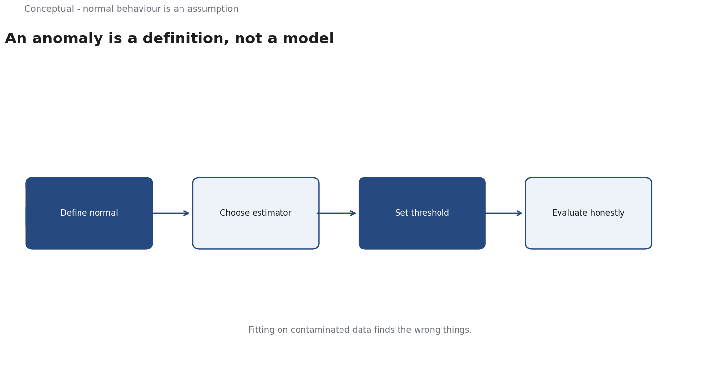
- Name the anomaly and its cost in business terms before choosing a method.
- Decide which of the three questions you are answering — outlier, novelty, or change.
- Build a simple baseline — a distributional method or Isolation Forest — and measure it.
- Check the API semantics of the estimator you use, especially for novelty scoring.
- Split before fitting and respect chronology for time-ordered data.
- Choose the threshold from the cost ratio, and record the reasoning.
- Monitor the alert rate as a first-class signal, because reviewer fatigue destroys the system.
For the pipeline discipline this depends on, see MLOps; for monitoring after deployment, see Model Monitoring.
A counterargument
A fair objection is that the article's "name the anomaly and its cost first" framing assumes the cost of each error type can be written down as a stable number - which is precisely what is hard in the fast-moving settings where anomaly detection matters most. scikit-learn's own documentation is hedged: Isolation Forest and neighbour-based methods "perform reasonably well on the data sets considered here," and One-Class SVM is "sensitive to outliers" - phrasing that signals dataset-specific results, yet the practical sequence tells readers to pick a threshold from a cost ratio as if those costs were knowable in advance. Hidden Technical Debt argues that production ML fails for organisational reasons, suggesting the real obstacle is glue code and monitoring, none of which a cleaner definition supplies. The "baseline usually wins" conclusion may understate cases where the definition itself must be learned from data.
References & Further Reading
- scikit-learn developers, 2026. Outlier detection with scikit-learn — How the classic unsupervised outlier detectors are actually implemented and when each one fails.
- scikit-learn developers, 2026. Common pitfalls and recommended practices (scikit-learn) — Data leakage, overfitting, and preprocessing mistakes that quietly inflate reported accuracy.
- D. Sculley et al., 2015. Hidden Technical Debt in Machine Learning Systems — Why production ML fails for organisational reasons rather than algorithmic ones.