Model Monitoring: Detecting Drift, Bias, and Performance Degradation
Drift, concept drift, and performance decay are different failures with different evidence. Learn what to measure, what to trust, and how to alert.
"Monitor your model" is advice that sounds like a responsibility and is actually an underspecified instruction. Monitor it for what? There are at least three distinct failures here, and they need different evidence: the inputs have changed, the relationship between inputs and outputs has changed, and the model's output quality has fallen. A signal that detects one will not detect the others, and a dashboard that conflates them gives false confidence in exactly the situations where you need it.
Direct answer: Drift monitoring asks whether the input distribution has moved. Concept monitoring asks whether the relationship between inputs and the target has moved — the one failure that actually changes the model's correctness, and the one that is hardest to see without labels. Performance monitoring asks whether measured quality has fallen. The reliable design is to instrument all three, to be explicit about which signal triggers which action, and — because production labels usually arrive late — to use input-distribution signals as an early warning for a quality signal you cannot yet observe.
Model monitoring is three separate disciplines.
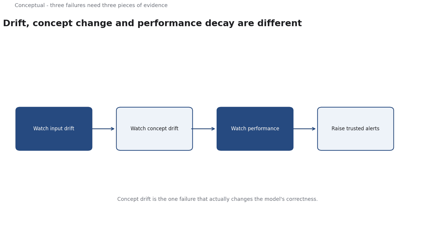
Three failures, three different pieces of evidence
The confusion is worth naming precisely, because the three failures have different latencies and different consequences.
Input drift is a change in the distribution of the features. It is directly observable at serving time, without labels, and it is the earliest signal you will get. It is also the weakest evidence on its own: a shift in the input distribution does not imply the model is wrong. It implies the model is operating in unfamiliar territory.
Concept drift is a change in the relationship between features and the target. The inputs look the same, the answer changed. This is the failure that makes a model wrong, and it is invisible to input monitoring by construction — by definition, the input distribution did not move.
Performance decay is the observable consequence: measured accuracy, error rate, or calibration has fallen. It is the most decision-relevant signal and the least available, because measuring it requires ground-truth labels, and labels arrive late — sometimes days, sometimes never for unlabelled traffic.
The design implication is that you cannot wait for performance signals. You instrument input drift as an early warning system for concept drift, and you treat the gap between the two as a risk to be sized rather than a problem to be solved.
Measuring drift without fooling yourself
The first discipline is the easiest to implement and the easiest to implement badly. Two failure modes dominate.
You leak the label. If the monitoring features are computed from a table that includes the target — or from any downstream transformation of it — then your drift metric is partly a proxy for the label, and your "early warning" is really a delayed performance signal with extra steps. The rule from the pipeline side applies here too: split first, fit nothing on the future, and keep the monitoring computation in the same object as the serving computation so the two cannot drift apart.
You alert on the wrong thing. A distribution statistic that moves is a signal to look, not a decision. The useful form of a drift alert names the action it triggers. If a feature's distribution shifts, what happens — retrain, route to a fallback, disable a segment, or page someone? An alert with no mapped action trains the team to ignore alerts.
For the mechanics, scikit-learn's outlier-detection documentation is a good source of concrete guidance because it compares estimators on their actual behaviour rather than in the abstract. It reports that "IsolationForest and neighbors" — the local-density-based methods — "perform reasonably well on the data sets considered here", and it is blunt about the alternative: "OneClassSVM is known to be sensitive to outliers and thus does not perform very well for outlier detection", requiring "fine-tuning of its hyperparameter nu to handle outliers and prevent overfitting". For scale, "SGDOneClassSVM provides an implementation of a linear One-Class SVM with a linear complexity in the number of samples."
There is a practical trap in that documentation worth internalising because it bites people in production. LocalOutlierFactor "does not support predict, decision_function and score_samples methods by default but only a fit_predict method, as this estimator was originally meant to be applied for outlier detection." A monitoring job that wants per-row scores from LOF needs the novelty-detection variant instead of the default one. This is exactly the kind of detail that turns "we monitor outliers" into a broken job at 03:00.
Detecting concept drift, and the proxy problem
Concept drift cannot be measured directly without labels. So monitoring systems use proxies, and the quality of the proxy determines everything.
The proxy you have at serving time is the model's own output distribution. If the model starts predicting a class it almost never predicted, something changed upstream. The weakness is circularity: the proxy is generated by the model you are trying to monitor, so a confidently wrong model produces a confident, unremarkable output distribution. Proxies detect unusualness, not error.
The second class of proxy uses the inputs: drift in the feature distribution, drift in the volume or shape of traffic, drift in the mix of request types. These are model-independent, which makes them more trustworthy as warnings, but they are one step removed from quality.
The third class is delayed truth: when labels do arrive, use them. The work here is not statistical, it is operational — you need a way to join a prediction to its eventual label, a way to evaluate the prediction using exactly the same feature computation as at serving time, and enough of a delay buffer that you are not evaluating on a partially-labelled population and calling the result a degradation.
Sculley et al. place this in the wider taxonomy of production ML failure: "boundary erosion, entanglement, hidden feedback loops, undeclared consumers, data dependencies, configuration issues, changes in the external world, and a variety of system-level anti-patterns". "Changes in the external world" is the drift case. The rest are the reason your drift detector may itself be broken — if the feature is computed in two places and one of them changes, you have a monitoring artefact that no longer describes the serving system.
Turning signals into alerts that people trust
The alerting problem has been solved for services and the solution transfers directly.
Google's site reliability guidance introduces burn rate as the core idea: "Burn rate is how fast, relative to the SLO, the service consumes the error budget." The worked example is unambiguous — a service with "a burn rate of 1" consumes budget at a rate that "leaves you with exactly 0 budget at the end of the SLO's time window", and "1% error rate uses exactly all of the error budget: a burn rate of 1."
That is the model to copy for model quality. Define an acceptable quality level as an SLO — say, an error rate on a 30-day window. A burn rate of 1 exhausts the allowance exactly at the end of the window; a burn rate of 10 exhausts it in three days. The alerting guidance then applies: alert on the burn rate, so that a slow drift does not page anyone and a fast one pages immediately. The short-window and long-window burn-rate alerts that service teams use map directly onto "short-window drift" and "long-window quality" signals.
The benefit is behavioural as much as statistical. A single threshold on a drift statistic produces a stream of alerts that drift slowly across, and the team learns to dismiss them. A burn-rate scheme produces few alerts, each of which means something.
Two rules make the scheme work. First, every alert must have a mapped action — retrain, roll back, fall back to a rules path, or investigate. Second, the action must be possible: a retraining trigger you cannot execute within the burn-rate window is a monitoring system that documents failure rather than preventing it.
Bias is a different question from drift
Bias monitoring is often filed under "model monitoring", but it fails for a reason the others do not: bias is not necessarily a change.
A model can be biased from deployment and never drift. It can also drift from an unbiased state into a biased one. Monitoring bias therefore requires a permanent measurement against a defined group, not a change-detection alarm on a group statistic.
The evidence required is the same evidence you would produce for an audit: performance reported by relevant group, including intersectional groups where the application calls for it. Model cards are the format for this, because they "provide benchmarked evaluation in a variety of conditions, such as across different cultural, demographic, or phenotypic groups ... and intersectional groups" relevant to the intended application, and they disclose "the context in which models are intended to be used". Datasheets do the dataset-side equivalent, documenting "its motivation, composition, collection process, recommended uses".
A disparity that is stable is a decision you have to make, not a fluctuation you wait out.
A monitoring design you can actually run
- Separate the three signals in the data model. Drift, concept-proxy, and measured quality are different columns with different owners. Conflating them makes the dashboard unreadable.
- Keep the monitoring computation identical to the serving computation. Share the code path, not a copy of it. This is what prevents the "monitoring says the data is stable while the model degrades" failure.
- Make drift a warning and quality a decision. Input drift triggers investigation; measured quality triggers action.
- Use burn rate, not fixed thresholds, so that slow drift is quiet and fast drift is loud. Define the quality SLO first and derive the windows from it.
- Map every alert to an action, and confirm the action is executable inside the window you chose.
- Measure group performance permanently, against the groups the application affects, and treat a stable disparity as a decision.
- Plan for delayed labels. Decide now how predictions will be joined to outcomes, because retrofitting it during an incident will not work.
For the pipeline contracts that have to hold before any of this is meaningful, see MLOps: From Experiment to Production Pipeline, and for the limits that make this hard, see The Limits of AI.
For an applied example of regression monitoring with a run registry and an investigate node that fires when accuracy drops, see the BTC Monthly ML case study.
A counterargument
The article borrows SRE burn rate as "the model to copy for model quality," but the analogy breaks on its own premise. Error budgets assume a signal observable inside the window; here labels arrive late or never, and the piece warns against evaluating on a partially-labelled population, so a 30-day quality SLO can measure an incomplete outcome. The early warning is weaker than presented: input drift "does not imply the model is wrong," and the output proxy "detects unusualness, not error," so it may fire on harmless shifts and miss the concept drift it should catch.
The objection is that a framework designed for services is applied to a signal far less observable than the one it was built for.
References & Further Reading
- D. Sculley et al., 2015. Hidden Technical Debt in Machine Learning Systems — Why production ML fails for organisational reasons rather than algorithmic ones.
- scikit-learn developers, 2026. Common pitfalls and recommended practices (scikit-learn) — Data leakage, overfitting, and preprocessing mistakes that quietly inflate reported accuracy.
- scikit-learn developers, 2026. Outlier detection with scikit-learn — How the classic unsupervised outlier detectors are actually implemented and when each one fails.
- Google, 2016. Alerting on SLOs — How to alert on symptoms and burn rate rather than on causes.