Batch Inference Economics: Throughput vs Latency
Batching raises throughput and can raise latency at the same time. Read the mechanism, a worked queue example, and how to choose an SLO.
A serving system can be fast for one request and inefficient for a thousand, or the reverse. Batching — grouping requests so the hardware processes them together — is the lever that trades latency for throughput. Understanding that trade is necessary before choosing either a model or a serving framework.
Direct answer: Batch inference processes multiple requests in one pass, increasing throughput because the hardware is used more fully, while adding waiting time as requests accumulate into a batch. The vLLM/PagedAttention paper describes how continuous batching and memory management raise serving throughput. The boundary: the right batch size depends on the latency your users will accept, which is a product decision, not a hardware setting.
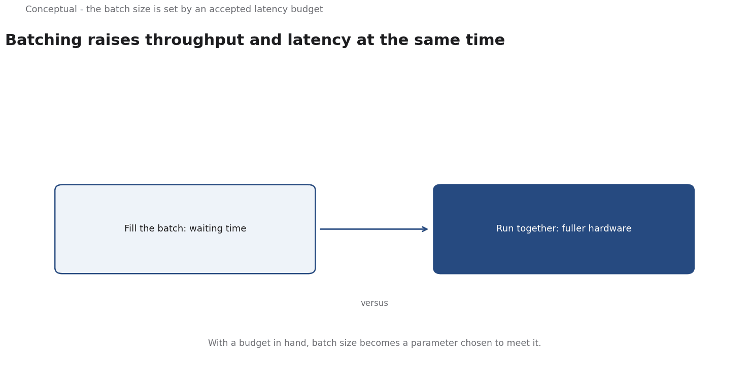
The trade-off
Three variables interact:
Arrival rate. Requests per second arriving at the system.
Batch size. How many requests are processed together. Larger batches use hardware better but take longer to fill.
Service time. How long a batch takes to process, which grows less than proportionally with batch size until memory or bandwidth saturates.
Two metrics describe the outcome:
- Throughput — requests completed per second, which determines cost per request at fixed hardware cost.
- Latency — time from arrival to response, especially the tail that users experience.
They move in opposite directions in the region where batching matters.
A worked queue example
The following is hypothetical and illustrative.
A model takes 40 ms to process one request alone. With a batch of 16, it takes 160 ms total — 10 ms per request on average. Requests arrive at 100 per second.
Batch of 1: Each request starts immediately and finishes in 40 ms. Throughput is limited by one-at-a-time processing — roughly 25 requests per second, far below the arrival rate, so a queue grows.
Batch of 16: Once 16 requests accumulate, processing takes 160 ms. Throughput rises to 100 requests per second, matching arrivals. But a request that arrives just after a batch fills waits up to 160 ms for the next one, plus its share of processing — tail latency around 200 ms.
Three lessons follow:
- The larger batch matches demand and prevents an unbounded queue, which the SRE error-budget article explains as a reliability concern.
- The tail latency is higher, which matters for interactive applications.
- The right choice depends on the SLO — a user-facing chat may need small batches; an offline document job can use large ones.
The arithmetic is simplified — real systems use continuous batching, which the serving-frameworks article covers — but the trade-off is the same.
Where batching pays
Offline and asynchronous work — document processing, analysis, evaluation — where latency is not user-visible.
High-volume endpoints with flexible latency requirements, where throughput determines cost per request.
Evaluation harnesses running thousands of prompts, as the evaluation article describes.
Where it hurts
Interactive applications where the user waits for each response.
Bursty traffic where batches fill unevenly and tail latency spikes.
Mixed workloads where a long request holds a batch and delays short ones, which is why request-length bucketing exists.
Faster hardware makes both paths faster; the relative tension between throughput and latency remains, which the GPU article explains at the hardware level.
Setting a latency budget
A useful latency budget starts from the user experience and works backwards. Three steps:
Choose a target percentile.
The median hides the experience of the slowest requests.
Pick a tail percentile — commonly the 95th or 99th — that reflects when users notice or abandon, as the SRE article explains for service objectives.
Allocate the budget. Split the target across components: network, queueing, prefill, and decoding. A 2-second budget might allow 100 ms of network, 200 ms of queueing, and the rest to generation. An allocation makes trade-offs visible.
Measure the queue separately. Queue time is the clearest sign of overload and the component most affected by batch size. An alert on queue growth gives the system a chance to shed load before latency becomes unacceptable, which the observability article covers.
With a budget in hand, batch size becomes a parameter chosen to meet it rather than a number picked for throughput in isolation.
What the metrics miss
Cost per request is not cost per useful answer. A larger batch may raise throughput while a different model raises accuracy, as the cost estimator explains.
Tail latency matters more than average. A few slow responses shape user perception, which the observability article covers.
Queues amplify failures. If the system cannot keep up, the backlog grows and older requests become useless — a failure mode the SRE article calls a latency outage.
A decision test
- Measure arrival rate and request-length distribution.
- State the latency SLO, including the tail, for each workload.
- Measure throughput and latency at several batch sizes.
- Separate interactive from batch traffic where possible.
- Price cost per request at the chosen operating point.
- Watch the queue as an early warning of overload.
- Re-measure after a model or hardware change.
For the serving mechanism, see Serving Frameworks; for the hardware, see Why GPU Computing Is Becoming a Strategic Resource.
References & Further Reading
- Woosuk Kwon et al., 2023. Efficient Memory Management for Large Language Model Serving with PagedAttention — Continuous batching and paged KV-cache memory that raise serving throughput.
- OpenAI, 2026. Models | OpenAI API — The GPT-6 lineup with published per-million-token input and output prices, context windows, reasoning levels and knowledge cutoffs.