Deep Learning Basics: Neural Networks, Backpropagation, and Practical Use Cases
A neural network is a composition of differentiable functions trained by following gradients. Read the mechanism, the scaling evidence, and when classical models still win.
Deep learning is often explained with metaphors — layers as "neurons", networks that "learn" — and the metaphors obscure a simple mechanism. A neural network is a chain of mathematical functions with adjustable parameters. Training means nudging those parameters in the direction that reduces a loss, using derivatives computed efficiently by backpropagation. Everything else — attention, distillation, scaling laws — is a refinement of that loop.
Direct answer: A network learns by composing simple transformations, measuring the error at the output, and propagating the gradient of that error back through the chain to update each parameter. The approach works when there is enough data and structure for the learned representations to help, and the empirical scaling literature shows that performance improves predictably with model size, data, and compute. The boundary: scaling laws are measured on cross-entropy loss for language modelling, not on your task, and deep learning loses to simpler methods on many tabular problems.
The mechanism, without the mysticism
A single layer computes a weighted sum of its inputs, adds a bias, and passes the result through a nonlinearity. Stacking layers composes these operations, and the composition can represent highly nonlinear functions — this is the sense in which depth gives a network more expressive power than a shallow model of the same width.
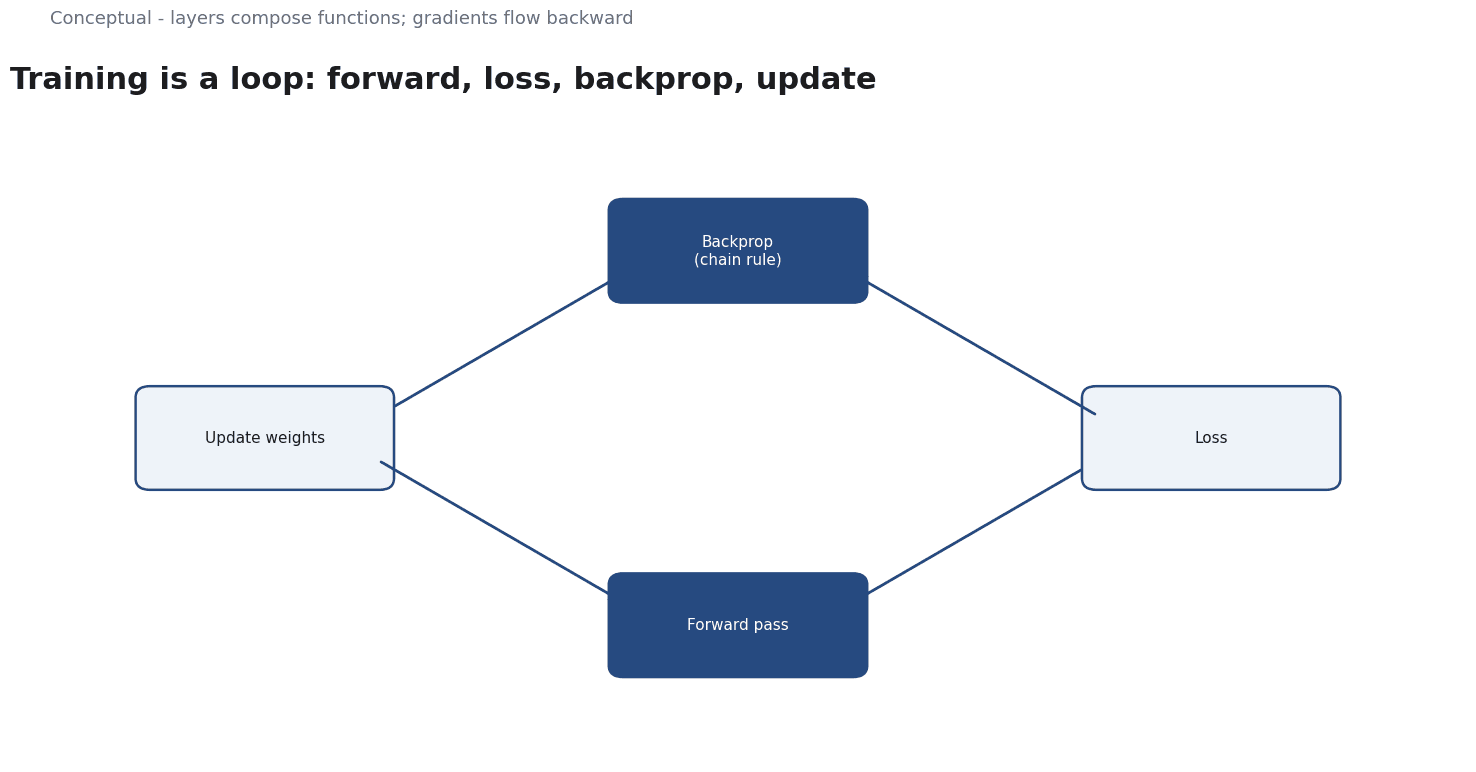
Three pieces make training work.
A loss function turns the network's output into a single number measuring error. For classification this is typically cross-entropy; for regression, squared error. The choice matters because it defines what "better" means.
Gradient descent updates each parameter in the direction that reduces the loss. The gradient tells you the slope; a learning rate controls how far you step. Too large and training diverges; too small and it never arrives.
Backpropagation computes those gradients efficiently. It applies the chain rule layer by layer from the output backward, reusing intermediate results so the cost is roughly proportional to the cost of a forward pass — not to the number of parameters times the number of paths. Without that efficiency, training deep networks would be impractical.
A useful consequence: a network does not "store" facts in the way a database does. It encodes regularities in the weights, distributed across many parameters. This is why a trained model can generalise to inputs it has never seen, and why it can fail in ways that are hard to localise.
Why depth and scale helped
The field's empirical regularities are captured in the scaling literature. Kaplan et al.'s "Scaling Laws for Neural Language Models" describe power-law improvements across model size, dataset size, and compute, while Hoffmann et al.'s later work — Chinchilla — found that many large models were "significantly undertrained" because the focus was on "scaling language models whilst keeping the amount of training data constant", concluding that "model size and the number of training tokens should be scaled equally".
Two technical developments made the larger models trainable. The transformer architecture of Vaswani et al., "Attention Is All You Need", replaced recurrence with attention over all positions, allowing parallel computation across a sequence — a prerequisite for training at scale. Residual connections, from the ResNet line of work, made very deep networks optimisable by letting layers learn modifications of their inputs rather than full transformations.
Distillation, from Hinton et al., addresses the deployment side: an ensemble can be too expensive to serve, and "it is possible to compress the knowledge in an ensemble into a single model which is much easier to deploy" by training the smaller model on the larger model's soft outputs. The student inherits some of the teacher's behaviour at a fraction of the inference cost.
A worked example of the training loop
Suppose you train a classifier on 50,000 examples in batches of 256, for 10 epochs. The arithmetic sets the real cost.
- Batches per epoch: 50,000 / 256 ≈ 195.
- Total updates: 195 × 10 = 1,950.
- If each batch takes 0.2 seconds on your hardware, one epoch is roughly 39 seconds and the run is about 6.5 minutes.
Now change one thing. Doubling the batch size to 512 halves the number of updates to about 975, but each update processes twice as much data, so the wall-clock time barely changes — while the memory requirement doubles. This is the common surprise: batch size is usually a memory and optimisation-stability decision, not a speed decision.
The learning rate interacts with this. A larger batch gives a lower-variance gradient estimate, which often permits a larger learning rate, but the safe range depends on the model and optimiser. The point is that the "hyperparameters" are not arbitrary settings; they are knobs on a specific numerical procedure with predictable trade-offs.
For tabular data, the comparison matters. A gradient-boosted tree model on 50,000 rows can often be trained in seconds, needs less preprocessing, and is easier to interpret. Deep learning earns its cost when the input has structure the network can exploit — images, text, audio — or when transfer learning from a pretrained model gives a head start.
Where deep learning loses
Three limitations deserve more than a disclaimer.
Data and compute are real constraints. Scaling laws describe what happens given more compute and data; they do not provide them. For a small dataset, a deep model will typically underperform a well-tuned classical method because it has enough capacity to memorise the training set.
The objective is a proxy. Cross-entropy on held-out text is not the same as usefulness, safety, or correctness on your task. The scaling papers optimise loss; downstream gains are supportive evidence, not the target.
Interpretability lags capability. A network's decision can be probed but not easily read off its weights. In regulated or high-stakes settings, that matters: the model card discipline of documenting evaluation conditions and known limits is not optional paperwork when you cannot fully explain a prediction.
On the other side, the strongest counterargument to "just use classical methods" is representation learning. On unstructured data, hand-engineered features are hard to beat, and pretrained deep models let a small team start from features learned on a much larger corpus.
The honest position is task-dependent, not ideological.
A decision test
Choose deep learning when the input has exploitable structure, when a pretrained model exists for the domain, or when the scale of data makes hand-engineered features the weaker option.
Prefer classical methods for small tabular datasets, when interpretability is required, or when the training budget is tight.
- Establish a simple baseline first — logistic regression or gradient boosting — so the deep model must earn its complexity.
- Check the data volume and structure against what the architecture needs.
- Use transfer learning before training from scratch.
- Track loss and the task metric separately so proxy improvements are not mistaken for progress.
- Estimate the full cost — training, inference, and maintenance — not just the experiment.
- Document evaluation conditions and limits alongside the model.
For how these models are trained and served reliably, see MLOps; for the compute question, see Why GPU Computing Is Becoming a Strategic Resource.
References & Further Reading
- Jared Kaplan et al., 2020. Scaling Laws for Neural Language Models — The empirical scaling relationships behind compute-optimal training.
- Jordan Hoffmann et al., 2022. Training Compute-Optimal Large Language Models — The compute-optimal allocation between parameters and training tokens.
- Ashish Vaswani et al., 2017. Attention Is All You Need — The transformer architecture that the NLP and LLM sections build on.
- Geoffrey Hinton, Oriol Vinyals, and Jeff Dean, 2015. Distilling the Knowledge in a Neural Network — Soft-label distillation, the basis of most model compression work.