How AI Models Are Trained: From Data to Deployment
Training a model is a chain of budget decisions, not a checklist. Learn how data, architecture, compute allocation, evaluation, and deployment each constrain the last.
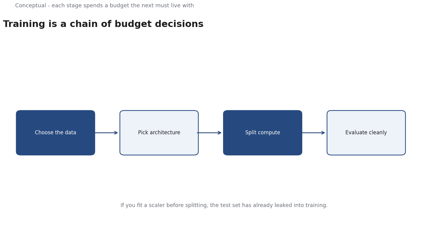
Most explanations of model training are a list of stages, and the list is the problem. It reads as if the stages were independent, when in practice each one spends a budget that the next one then has to live with. Data choice constrains what the model can learn. The compute budget constrains which architecture is even worth training. The evaluation design constrains which numbers you are allowed to believe.
Direct answer:
Training is a sequence of budget decisions: how much data to collect and how to document it, which architecture to instantiate, how to split a fixed compute budget between model size and training tokens, how to evaluate without leaking information, and what to ship.
Every stage can invalidate the last one. The most common failure is not a bad model — it is a good model measured on a broken split, or a well-trained model that was never a good idea to deploy. The paper that most usefully reframes the whole process is the compute-optimal training study, because it shows that the popular instinct — make the model bigger — is frequently the wrong allocation of a fixed budget.
Where the ceiling is set: the data
Data is usually described as the input to training. It is more accurately the ceiling on what training can achieve, and it is also the part of the pipeline most often undocumented.
Gebru et al. proposed datasheets for datasets by analogy with electronics: every component ships with a datasheet describing its operating characteristics, test results, and recommended uses, and they argue a dataset should ship with the equivalent — its motivation, composition, collection process, recommended uses, and known limits. The problem they set out to solve is that the machine learning community has no standardised process for documenting datasets, and that this "can lead to severe consequences in high stakes domains". That is a claim about evidence, not about sentiment: a dataset nobody documented is a dataset whose provenance nobody can reconstruct.
Mitchell et al. make the complementary argument for models, proposing model cards — short documents accompanying trained models that report benchmarked evaluation "in a variety of conditions, such as across different cultural, demographic, or phenotypic groups ... and intersectional groups" relevant to the intended application. Their motivation is equally concrete: trained models are used for tasks "in areas such as law enforcement, medicine, education, and employment", where intended-use context and evaluation procedure are part of the artefact, not optional metadata.
The practical consequence for a team: a dataset card and a model card are not paperwork. They are the only artefacts that let a later reader tell the difference between a model that is accurate and a model that is accurate on the distribution someone happened to collect.
Architecture: what the transformer actually changed
Architecture choice is usually justified by pointing at a leaderboard. The original transformer paper is more useful because it explains what the architecture enabled.
Vaswani et al. proposed a network "based solely on attention mechanisms, dispensing with recurrence and convolutions entirely", and the reason it won was not only quality but parallelism: on WMT 2014 English-to-German the model reached 28.4 BLEU, improving on previous best results "including ensembles by over 2 BLEU", and on English-to-French it set a single-model state-of-the-art 41.8 BLEU "after training for 3.5 days on eight GPUs, a small fraction of the training costs of the best models from the literature". The paper then generalised the model to English constituency parsing, with both large and limited training data.
Two things follow. The quality-per-compute gain is real, and it is why transformers displaced recurrent stacks — but the gain was measured on translation, and transferring it to a new domain is an assumption you have to test, not a law. And the paper frames this as an efficiency result as much as a quality result. When you read a leaderboard entry, ask what it cost.
The compute allocation: the finding that changes the decision
This is where the popular instinct and the evidence diverge.
Kaplan et al. studied empirical scaling laws and found that the loss "scales as a power-law with model size, dataset size, and the amount of compute used for training, with some trends spanning more than seven orders of magnitude", while "other architectural details such as network width or depth have minimal effects within a wide range". Their optimisation conclusion was that compute-efficient training involves "training very large models on a relatively modest amount of data and stopping significantly before convergence". On that reading, a bigger model is the efficient choice.
Hoffmann et al. re-examined the allocation under a fixed compute budget and reached a different conclusion. They trained "over 400 language models ranging from 70 million to over 16 billion parameters on 5 to 500 billion tokens", and found that "for compute-optimal training, the model size and the number of training tokens should be scaled equally: for every doubling of model size the number of training tokens should also be doubled". Their diagnosis was that existing large models were "significantly undertrained, a consequence of the recent focus on scaling language models whilst keeping the amount of training data constant".
They then tested it: Chinchilla, a predicted compute-optimal model with 70B parameters trained on 4× more data than Gopher at the same compute budget, "uniformly and significantly outperf[o]rmed Gopher (280B), GPT-3 (175B), Jurassic-1 (178B), and Megatron-Turing NLG (530B) on a large range of downstream evaluation tasks". On MMLU it reached "a state-of-the-art average accuracy of 67.5%, greater than a 7% improvement over Gopher".
The decision this changes is concrete. Under a fixed budget, halving the parameter count and doubling the tokens is a different experiment from keeping the parameter count and training longer. The popular path — scale the model, keep the data roughly constant — is the one the compute-optimal work identifies as undertrained. The detailed treatment of how these two studies conflict is in Chinchilla and the Scaling Laws.
Evaluation: the stage that silently invalidates the others
A model that scores well on a broken evaluation tells you nothing about the model. scikit-learn's guidance on data leakage is the cleanest statement of the failure mode: "Data leakage occurs when information that would not be available at prediction time is used when building the model." Their remedy is blunt — "Always split the data into train and test subsets first, particularly before any preprocessing steps" — and they note that a pipeline "ensures that the appropriate method is performed on the correct data subset".
That last point is the one teams skip.
The symptom is a validation score that looks wonderful and a production score that does not.
Broader evaluation is a separate job, and it is where model cards earn their place: reporting performance across demographic and other relevant groups, disclosing intended use, and describing the evaluation procedure, rather than reporting one headline metric on one aggregate.
Deployment: the stage that changes the model
A trained model is not the deliverable. Hinton et al. showed the shape of the trade-off in a direction people often forget — the constraint at deployment is usually serving cost, not accuracy. Their approach compresses an ensemble into a single model "which is much easier to deploy", reporting "some surprising results on MNIST" and a "significant" improvement to "the acoustic model of a heavily used commercial system" by distilling an ensemble into one model.
That is the pattern for most production inference: the accuracy you validated was produced by something more expensive than what you can serve. Distillation, quantisation, or a smaller architecture are not accuracy sacrifices in the abstract — they are decisions about which part of the validated capability to keep.
And then the model is in production, where the failure modes are not the ones the training loop optimised. Sculley et al. catalogued the "hidden technical debt in machine learning systems", and the recurring theme is that most of the work is not the model: data collection, feature extraction, serving infrastructure, and monitoring. The upstream consequence is organisational rather than algorithmic, which is why adoption so often stalls after the model works.
A repeatable check you can run this week
Before you believe any training result, walk these five questions and answer them with artefacts rather than opinions:
- Can someone else rebuild this split? Produce the training/validation/test partition and confirm that every preprocessing step was fitted inside the training fold only. If you cannot show it, assume leakage.
- What did the compute actually buy? Write down the parameter count, the token count, and the budget. If tokens did not scale roughly with parameters, you are in the undertrained regime the compute-optimal work describes.
- Does the dataset have a datasheet and the model a card? If not, write them before publishing — most of the content is already in your head and in the notebooks.
- What is the serving cost of the thing you validated? If the validated artefact was an ensemble and you intend to ship one model, measure the gap you are accepting.
- What breaks first in production? Name the monitoring signal — input distribution shift, latency, error rate, or a quality proxy — and who gets paged. If the answer is "we will look at the dashboards", the pipeline is not finished.
For the organisational side of this — why a working model so often fails to reach users — see Why AI Adoption Is Harder Than Building an AI Model.
A worked example
The following is hypothetical and illustrative. A team plans to train a language model under a fixed compute budget and audits the plan first. Check one, can the split be rebuilt: the training, validation, and test partition is written down and every preprocessing step is fitted inside the training fold, following the leakage rule scikit-learn states, because a scaler fitted on the full set lets the test set leak into training. Check two, what did the compute buy: the team records parameter and token counts and finds tokens scaled with parameters, matching Hoffmann et al.'s compute-optimal allocation; an undertrained large model would be the wrong allocation of the same budget. Check three, what is the serving cost of the validated artefact: if the tested model is an ensemble but a single model must ship, the team measures the accuracy gap that distillation, as Hinton et al. describe, would accept, and names the production monitoring signal. The bounded outcome is a budget spent on a reproducible split, a token count that matches the model, and a deployable artefact with a known gap, recorded in a datasheet and model card.
A counterargument
A critic could argue that the budget-chain framing is tidier than the evidence it cites. The compute-optimal result is presented as the decision that changes everything, but Kaplan and Hoffmann disagree, and both settings are language modelling under a fixed training budget; Hoffmann's 'optimal' is defined by that budget, not by the serving constraint Hinton et al. say dominates deployment. Its deployment section undercuts the compute section: if the validated model is replaced by a distilled or quantised one, the earlier allocation is only part of the story. Sculley et al. go further, describing most of the work as data collection, serving, and monitoring rather than training.
The linear pipeline is a useful teaching device, but it flatters a process the cited sources describe as iterative and mostly non-model.
References & Further Reading
- Ashish Vaswani et al., 2017. Attention Is All You Need — The transformer architecture that the NLP and LLM sections build on.
- Jared Kaplan et al., 2020. Scaling Laws for Neural Language Models — The empirical scaling relationships behind compute-optimal training.
- Jordan Hoffmann et al., 2022. Training Compute-Optimal Large Language Models — The compute-optimal allocation between parameters and training tokens.
- Geoffrey Hinton, Oriol Vinyals, and Jeff Dean, 2015. Distilling the Knowledge in a Neural Network — Soft-label distillation, the basis of most model compression work.