Computer Vision Basics: CNNs, Transfer Learning, and Object Detection
Vision models learn spatial hierarchies. Read what each architecture changed, and why transfer learning is the default rather than the exception.
Computer vision converts pixels into representations a model can use. The field's history is a sequence of answers to a specific question: how do you build a representation that is useful across an image, robust to where an object appears, and cheap enough to train? The architectures people memorise are solutions to that problem, not arbitrary milestones.
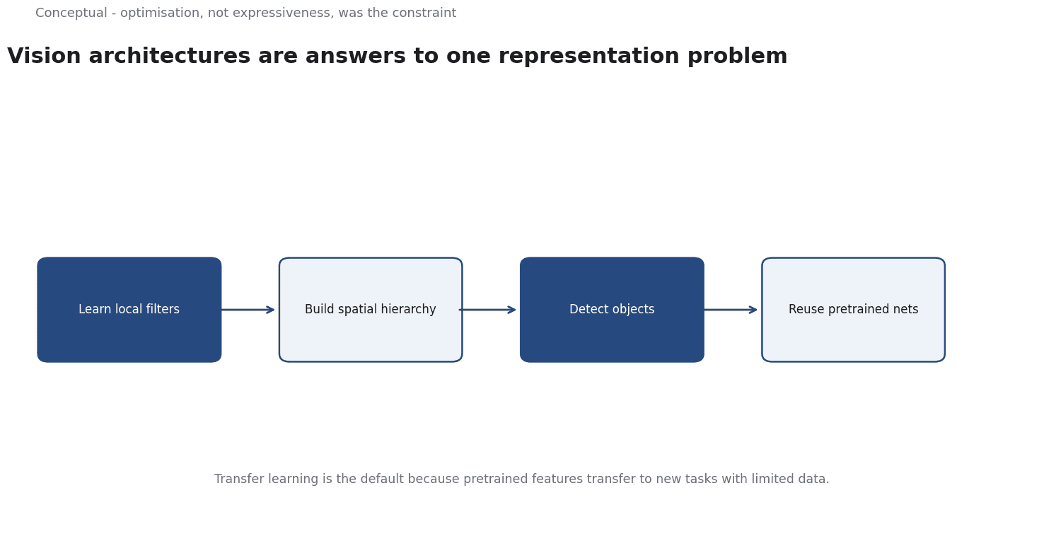
Direct answer: Convolutional neural networks learn spatial filters that build a hierarchy — edges, textures, parts, objects — while sharing weights across an image. ResNet made very deep networks trainable through residual connections; Faster R-CNN and YOLO represent the two-stage and single-stage approaches to detection; Focal Loss addressed the class imbalance that held single-stage methods back; and Vision Transformers replaced convolution with attention over image patches. Transfer learning is the default because pretrained features transfer well to new tasks with limited data, which is the situation most practitioners actually face.
Why convolution works
Convolution addresses both problems.
A filter — a small window of weights — slides across the image and produces a response at each location. Three properties follow:
Local connectivity. Each output depends on a small region, which matches the structure of visual features: an edge is a local phenomenon.
Weight sharing. The same filter is applied everywhere, so a pattern learned in one part of an image is recognised in another, and the parameter count does not grow with image size.
Hierarchical composition. Stacking layers with pooling builds increasingly abstract features. Early layers respond to edges and textures, middle layers to parts, and later layers to objects. This is the spatial hierarchy the literature describes, and it is why depth matters.
Pooling reduces spatial dimensions and provides a degree of translation invariance — moving an object slightly changes the pooled representation less than it changes the raw pixels. It also increases the receptive field of later layers, so each unit sees more of the input.
What ResNet changed
Depth helps until it does not: adding layers beyond a point makes training harder, with accuracy degrading rather than improving. He et al.'s solution was the residual connection — a shortcut that lets a layer block learn a modification of its input rather than a complete transformation of it. Their paper, "Deep Residual Learning for Image Recognition", demonstrated that networks with 50 to 152 layers could be trained effectively, which is the structural claim behind the familiar depth numbers.
The general lesson is that optimisation, not expressiveness, was the constraint.
A deeper network could represent more; it was simply hard to train until the architecture made the identity mapping easy to learn.
Detection is a different problem
Classification assigns one label to an image. Detection must find multiple objects, localise them with bounding boxes, and classify each. That adds two difficulties: where to look, and how to handle the overwhelming number of background locations that contain no object.
The field split into two approaches:
Two-stage detectors, exemplified by Faster R-CNN, first propose candidate regions and then classify and refine them. Ren et al.'s "Faster R-CNN" introduced a region proposal network that made the proposal stage learned rather than hand-designed, which improved both speed and accuracy. The trade-off is two passes over the image, which costs latency.
Single-stage detectors, of which YOLO is the best-known, predict boxes and classes directly from the image in one pass. Redmon et al.'s "You Only Look Once" reframed detection as a single regression problem, which gave up some localisation accuracy in exchange for real-time speed. The approach made detection practical on video and embedded devices.
For years the trade-off seemed fixed: two-stage methods were more accurate, single-stage methods were faster. Lin et al.'s "Focal Loss for Dense Object Detection" changed that by addressing the class imbalance that hurts single-stage training — most candidate locations are easy negatives, and they dominate the loss. With focal loss, a single-stage detector could match two-stage accuracy while retaining its speed advantage.
The pattern is instructive: the bottleneck was not the architecture but the training objective, and a better loss function changed the comparison.
Transformers enter vision
Dosovitskiy et al.'s "An Image is Worth 16x16 Words" treated an image as a sequence of patches and applied a transformer to them, dispensing with convolution entirely. The result showed that attention-based models could match or exceed convolutional ones given enough data.
The practical difference is in inductive bias. Convolution assumes locality and translation invariance, which helps when data is limited. Attention makes fewer assumptions and can model long-range relationships, which helps at scale but requires more data to learn the structure that convolution builds in. Carion et al.'s DETR applied a transformer to detection directly, using set prediction with bipartite matching and removing the need for the non-maximum suppression step that had been a fixture of detection pipelines.
The field has not simply replaced convolution; it has expanded the set of tools, with hybrid designs common in practice.
Transfer learning is the default
Training a vision model from scratch requires a large labelled dataset and substantial compute. Most projects have neither. Transfer learning — starting from weights pretrained on a large dataset and adapting the final layers — is the standard approach because the early layers learn general features that transfer across tasks.
Three decisions matter:
- How much of the model to fine-tune. With a small target dataset, freezing the backbone and training only a new head reduces overfitting. With more data, unfreezing later layers improves adaptation.
- The learning rate. Pretrained weights are useful and should not be destroyed by a large update; a smaller rate for the backbone than for the new head is standard.
- Domain similarity. Features learned on natural photographs transfer poorly to medical images or satellite data when the low-level statistics are very different. The more distant the domain, the more fine-tuning is required.
The honest caveat is that pretrained models carry the biases and blind spots of their training data. A model pretrained on one population may underperform on another, which is why model cards call for evaluation across relevant groups.
A practical sequence
- Define the task precisely — classification, detection, or segmentation — because the architecture follows from it.
- Start with a pretrained model and a small fine-tuning setup.
- Establish a baseline before trying architectural changes.
- Inspect failures by category, not only the aggregate metric, because errors cluster in specific conditions.
- Choose detector architecture by the speed-accuracy point the application requires, not by leaderboard rank.
- Check the data distribution against the pretraining domain and fine-tune accordingly.
- Report performance by relevant subgroup, following the model-card discipline.
A worked example of detector selection
The choice between detector families becomes concrete with a latency budget. Suppose a system must process a video stream at 25 frames per second, giving 40 milliseconds per frame including preprocessing and inference.
A two-stage detector such as Faster R-CNN may offer strong localisation accuracy but require more than 40 milliseconds per frame on the available hardware. A single-stage model such as YOLO may process the frame in under 20 milliseconds with somewhat lower accuracy on small objects. Focal Loss narrows the accuracy gap without restoring the two-stage cost, because it improves training rather than adding a stage.
The decision is therefore not "which model is most accurate?" but "which model meets the accuracy floor inside the latency budget?" Three factors decide it:
- The size of the objects that matter. Small objects suffer most from the coarse grids used by single-stage detectors, so an application detecting distant pedestrians has a different accuracy floor from one counting pallets.
- The hardware. A model's speed is a property of the model and the device together, and a result from a data-centre GPU says little about an embedded processor.
- The cost of a missed detection. If missing an object is expensive, accuracy takes priority and the frame rate may need to be reduced; if the system is advisory, latency may dominate.
The same arithmetic applies to accuracy targets: a reported mean average precision averages across object sizes and conditions, and an application may care much more about one category. Reporting performance by category and by object size is more informative than a single number, and it is the vision equivalent of the model-card discipline.
For the evaluation framework, see MLOps; for the deployment constraints, see Edge AI.
A counterargument
A fair objection is that the article tells the field's history too neatly. Each architecture is presented as the rational answer to a stated bottleneck - "optimisation, not expressiveness, was the constraint" - which reads the outcome backwards into the motive. The cited results are more conditional than this allows: Dosovitskiy et al. show attention matching convolution only given enough data, and the article concedes convolution's inductive bias helps when data is limited while ViT needs more. Tan and Le's EfficientNet agrees, attributing gains to scaling depth, width, and resolution rather than any one architectural idea. The worked detector example admits speed is "a property of the model and the device together", then quotes millisecond figures as if stable.
References & Further Reading
- Kaiming He et al., 2016. Deep Residual Learning for Image Recognition — Residual connections, the architecture that made very deep CNNs trainable.
- Shaoqing Ren et al., 2015. Faster R-CNN: Towards Real-Time Object Detection with Region Proposal Networks — The two-stage detector that introduced region proposal networks.
- Joseph Redmon et al., 2016. You Only Look Once: Unified, Real-Time Object Detection — The single-stage detector that reframed object detection as a regression problem.
- Tsung-Yi Lin et al., 2017. Focal Loss for Dense Object Detection — The class-imbalance loss that made single-stage detectors work.
- Alexey Dosovitskiy et al., 2020. An Image is Worth 16x16 Words: Transformers for Image Recognition at Scale — The vision transformer that moved vision models beyond CNNs.
- Nicolas Carion et al., 2020. End-to-End Object Detection with Transformers — Set prediction with bipartite matching, removing the need for non-maximum suppression.
- Mingxing Tan and Quoc V. Le, 2019. EfficientNet: Rethinking Model Scaling for Convolutional Neural Networks — Compound scaling of depth, width, and resolution.