Missing Data: When Dropping Rows Changes the Answer
Missing values are encoded, and your handling of them changes the population you analyse. Read the drop-versus-impute trade-off and a worked bias example.
A model can look excellent in validation and fail in production because the training pipeline quietly deleted every row with a missing field. The validation set had the same deletions, so both measurements described a cleaner population than the one the model now serves. Nothing in the code was wrong; the decision to drop rows was just invisible.
Direct answer: Missing values are represented by sentinels such as NaN, NaT, None, or blanks, and each representation needs detection before anything else. scikit-learn notes that discarding incomplete rows "comes at the price of losing data which may be valuable (even though incomplete)" and that "a better strategy is to impute the missing values, i.e., to infer them from the known part of the data". The boundary: imputation creates values that were never observed, and no method can recover information that is absent — so the choice must match the reason the data is missing and the decision the analysis supports.
If higher earners were less willing to disclose, the missing rows are systematically different from the observed ones, and dropping them changes the population.
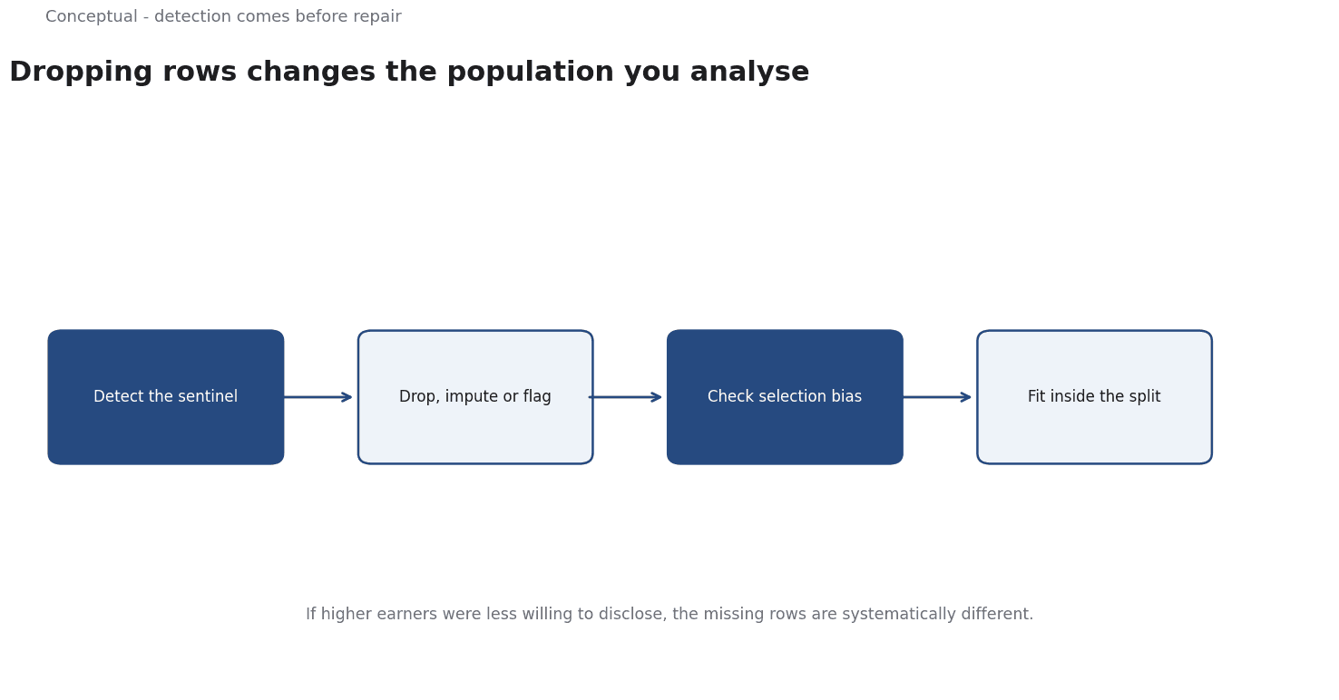
Step one is detection, not repair
pandas uses several sentinels rather than one: NaN for NumPy numeric types, NaT for datetimes, and <NA> for nullable extension types; None is also treated as missing. The documentation points to isna() and notna() as the detection methods.
This matters because a value that is not recognised as missing is worse than one that is. A blank string in a numeric column, a sentinel like -1, or a text marker such as "unknown" may survive into an analysis as a real observation. Three habits prevent the common errors:
- Check each column's missing rate before deciding anything, with the encoding documented.
- Distinguish structural absence — a field that cannot exist for a given row — from a value that failed to record.
- Treat the sentinel as data you chose, not a property of the source, when you convert or replace it.
Only after detection does the real question arise: what does the missingness mean?
Drop, impute, or flag
scikit-learn describes three broad approaches.
Discard rows or columns. The simplest option, and the one with the steepest cost when missingness is not random. It also removes rows that may be valuable precisely because the field is missing — a customer who declines to give an income is different from one whose income was recorded.
Univariate imputation. SimpleImputer fills missing values with a constant, or with the mean, median, or most frequent value of the column. It "imputes values in the ith feature dimension using only non-missing values in that feature dimension". Fast and predictable, but it ignores relationships between columns and compresses the distribution — every missing income becomes the same number.
Multivariate imputation. IterativeImputer "models each feature with missing values as a function of other features" in repeated rounds, using other columns to predict each missing value. The scikit-learn documentation labels this estimator experimental, noting that defaults and behaviour may change — a reason to pin versions and validate the result, not a reason to avoid it.
A fourth option is to keep the missingness itself as a signal: add an indicator column recording which values were absent, then impute. Whether that helps depends on whether absence carries information, which is an empirical question about your data.
A worked example of selection bias
The following numbers are hypothetical and illustrative.
A survey of 10,000 people asks for annual income. Two thousand leave the field blank. A team runs dropna() and computes the mean income of the remaining 8,000 respondents: 50,000.
Suppose — unobserved by the team — the 2,000 non-respondents would have reported an average of 35,000. The full-sample mean would be:
(8,000 × 50,000 + 2,000 × 35,000) / 10,000 = 47,000
The complete-case analysis overstates mean income by 3,000, or about 6.4%. Three observations follow:
- The bias comes from the reason for missingness, not from the deletion code. If higher earners were less willing to disclose, the missing rows are systematically different from the observed ones, and dropping them changes the population.
- Mean imputation does not fix it. Filling all 2,000 blanks with 50,000 preserves the biased mean by construction and shrinks the variance. It makes the dataset look complete while removing the evidence of a problem.
- A missing-indicator would surface it. Keeping a flag for income-not-reported lets the analysis show that the group exists and, if relevant, model it separately. That is more honest than inventing a value and pretending it was measured.
The correct response depends on the question. If the goal is the mean income of respondents who disclose, complete cases answer it. If the goal is the mean income of the population, a method that accounts for nonresponse is required, and the result must be labelled with that assumption.
The leakage trap in pipelines
scikit-learn's guidance on data leakage says a leak occurs when "information that would not be available at prediction time is used when building the model". Imputation is a fitted transformation: the mean or median is computed from data.
The remedy is mechanical: split first, then fit the imputer on training data only, and apply the same fitted transformation to validation and test data. A Pipeline that bundles imputation with the estimator enforces this ordering and makes it hard to apply the wrong transform to the wrong subset. The same rule applies to the missing-indicator: which columns are flagged should be decided from training data.
For time-ordered data the split must respect chronology, and imputation must use only values available at the prediction time — a rolling window, not future observations.
What imputation cannot do
Three limits should be explicit.
It does not create information. Every imputed value is an estimate from what remains. A column that is 60% missing cannot carry the same signal as one that is 5% missing, however sophisticated the method.
The mechanism matters. When missingness depends on observed variables, using those variables in imputation can help. When it depends on unobserved or unrecorded values, no method based on the available data can fully repair the bias — the missing values carry information that was never captured.
A clean-looking dataset can hide the problem. After imputation, downstream users see no gaps and may assume every value was measured. Keeping the indicator and documenting the missing rates is part of the deliverable, not optional cleanup.
The counterargument to careful handling — that a simple median fill worked well enough in practice — is sometimes true. It is defensible when the missing rate is low, the field is not central to the decision, and the missingness is plausibly unrelated to the outcome.
It is not defensible as an invisible default.
A decision test
- Detect the encodings per column and report missing rates before doing anything else.
- Name the reason for missingness as a hypothesis, and say what would falsify it.
- Ask which population the analysis claims to describe — respondents, or the wider population.
- Split before fitting any imputer, and keep it inside a pipeline.
- Compare at least two strategies — complete cases and one imputation method — and report whether the conclusion changes.
- Keep a missingness indicator when absence may be informative.
- Document the rates and the method alongside the result, so a reader knows which values were never observed.
For the pipeline discipline, see Python for Data Analytics; for the broader data context, see Why Data Quality Matters More Than Model Complexity.
References & Further Reading
- pandas developers, 2026. Working with missing data — pandas documentation — The different sentinels pandas uses for missing values — NaN, NaT, None and pandas.NA — and the isna/notna detection methods.
- scikit-learn developers, 2026. Imputation of missing values — scikit-learn documentation — Dropping versus imputing missing values, univariate vs multivariate imputation, and the experimental status of IterativeImputer.
- scikit-learn developers, 2026. Common pitfalls and recommended practices (scikit-learn) — Data leakage, overfitting, and preprocessing mistakes that quietly inflate reported accuracy.