Python for Data Analytics: Pandas, NumPy, and Visualization Workflows
The Python analytics stack shapes data and checks assumptions. Read the workflow that keeps analysis reproducible and the leakage trap that invalidates it.
Most Python analytics tutorials teach the API: how to call groupby, how to reshape a frame, how to draw a chart. The harder part is the workflow around the code — what gets computed from what, which transformations are fitted on which rows, and how a reader could reproduce the result. A clean analysis is mostly a set of decisions about order and provenance.
Direct answer: NumPy provides fast array operations, Pandas provides labelled tabular data structures, and a plotting library turns the results into something a human can inspect. The stack is powerful because the operations compose, and dangerous for the same reason: a transformation fitted on the full dataset can quietly leak information from the future or the test set into the model.
The defence is a pipeline that splits data before fitting anything and applies each transform to the correct subset.
What each tool actually contributes
NumPy stores homogeneous numeric data in contiguous arrays and performs vectorised operations on them. Vectorisation matters for performance because the loop runs in compiled code rather than in the Python interpreter. The mental model is an array of values with a shape, and operations that produce new arrays.
Pandas adds labels — row indices and column names — and heterogenous types. Its core structures, the Series and DataFrame, make operations like grouping, joining, and handling missing values expressible in a few lines. The convenience comes with a cost: the same operation can be written several ways with subtly different behaviour around missing data and index alignment.
Visualization is not decoration. A plot is a diagnostic: it reveals outliers, seasonality, and distribution shapes that a summary statistic hides. The choice of chart should follow the question — distribution, relationship over time, or comparison across groups — not the other way around.
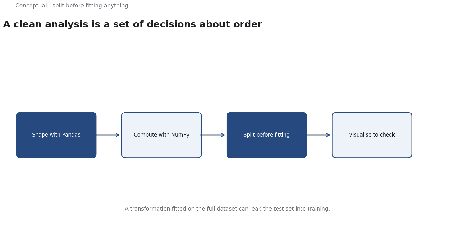
The three form a workflow: load and clean in Pandas, compute numeric operations with NumPy underneath, inspect the result with a plot, then formalise the check in a model or a test.
The workflow that keeps analysis honest
Four habits separate a reproducible analysis from a notebook that only made sense to its author.
State the question and the unit of analysis. A row in the frame is a customer, a transaction, or a day — and the answer means different things depending on which. Kuhn and Johnson's Feature Engineering and Selection is useful precisely because it insists on the modelling context: a feature's value depends on what you are predicting and when.
Split before preprocessing. scikit-learn's guidance is explicit: "data leakage occurs when information that would not be available at prediction time is used when building the model". If you scale, impute, or encode categories using statistics from the whole dataset, the held-out rows have influenced the transformation. The documentation's prescription is to split first and use pipelines so the correct transform is applied to the correct subset.
Keep the transformations in one place. A Pipeline object that bundles imputation, scaling, and the estimator makes it much harder to accidentally fit on the wrong rows. It also makes the analysis portable: the same object can be cross-validated and later deployed.
Pin the environment. A result computed with one library version may differ under another. Record the versions and the random seed; "it worked in my notebook" is not a reproduction.
A worked example of leakage
Suppose you are predicting customer churn from a table with a last_login column. You load the data, impute missing values with the median, standardise numeric columns, and split 80/20 into train and test. A cross-validated model reports 0.88 AUC, which looks excellent.
Now examine the order. The median and the scaling parameters were computed across all rows, including the test set. That is a small leak. The larger problem appears when you inspect the feature: last_login was recorded after the churn decision in many cases — customers who churned simply stopped logging in. The feature encodes the outcome, which is leakage of the more serious kind.
scikit-learn's definition applies directly: a value not available at prediction time was used to build the model. Two fixes are needed:
- Move the split before the transforms, and fit imputation and scaling on training folds only. A
PipelinewithColumnTransformerenforces this mechanically. - Redefine the feature using only information available at the prediction date — for example, login frequency in the 30 days preceding the cutoff, not the last login ever.
The 0.88 AUC was not measuring predictive skill. It was measuring how well the model could read a consequence of the outcome.
This is why a surprisingly good result is a reason to audit the pipeline, not to celebrate.
For time-ordered data the same rule applies with a sharper edge: use an expanding-window split such as TimeSeriesSplit, and respect the gap parameter when labels arrive late.
Visualization as a check, not a conclusion
Three plots earn their place in almost any analysis:
- A distribution plot of each important numeric column, to see skew, multimodality, and impossible values before they reach a model.
- A missingness map or count, to see whether missing values cluster in particular columns or time periods — missingness is often informative, and dropping it silently loses signal.
- A plot of the target against time or a key predictor, to reveal non-stationarity or a relationship that is not the one the summary statistic suggests.
The discipline is to make the plot, state what it shows, and then decide whether it changes the analysis. A chart that is produced and ignored is busywork.
The limits of the stack
Two cautions keep the toolkit in perspective.
Convenience hides assumptions. Pandas will silently align on index labels when you combine two series, which is helpful until two frames share an index by coincidence. Many analysis bugs are not exceptions; they are operations that succeeded on the wrong rows.
The library is not the method. Knowing the API does not tell you whether a cross-validation scheme matches the deployment question, whether a feature is available at prediction time, or whether an aggregate metric hides a subgroup failure. Those are decisions about the problem, and they matter more than syntax.
The relevant counterargument to "just use a pipeline" is that real exploration is messy and you often do not know the right transforms in advance. That is true. The answer is not to avoid pipelines but to treat exploratory analysis as hypothesis generation and then rebuild the result in a clean, ordered pipeline before reporting it.
A decision test
- Write the question and the prediction date at the top of the notebook.
- For every feature, ask whether its value existed at that date.
- Split before any fitted transform, and enforce it with a pipeline.
- Choose a validation scheme that mirrors deployment — random for independent rows, expanding window for time series.
- Plot distributions and missingness before modelling.
- Record versions and seeds so the result can be reproduced.
- Treat a surprisingly high score as a prompt to audit the ordering.
For the broader evaluation and monitoring discipline, see Model Monitoring; for the production handoff, see MLOps.
References & Further Reading
- scikit-learn developers, 2026. Cross-validation: evaluating estimator performance (scikit-learn) — Time-series splits and the validation design that keeps a backtest honest.
- scikit-learn developers, 2026. Common pitfalls and recommended practices (scikit-learn) — Data leakage, overfitting, and preprocessing mistakes that quietly inflate reported accuracy.
- Max Kuhn and Kjell Johnson, 2019. Feature Engineering and Selection: A Practical Approach for Predictive Models — The closest thing to a reference text on feature construction, resampling, and selection.