Mixture of Experts: Why Sparse Models Changed AI Economics
Sparse models route each token to a subset of parameters. Read the mechanism, the 671B/37B numbers, and the costs that do not disappear.
A dense language model uses all of its parameters for every token. A mixture-of-experts model uses only a few. That single change alters the economics of scaling: a model can have hundreds of billions of parameters while doing the per-token work of a much smaller one. It also introduces failure modes that dense models do not have.
Direct answer: A sparse mixture of experts (MoE) contains multiple expert subnetworks and a router that selects which experts process each token. Mixtral 8x7B's router "selects two experts to process the current state and combine their outputs" at each layer. DeepSeek-V3 reports "671B total parameters with 37B activated for each token". The boundary: sparsity reduces computation per token, not memory, communication, or training difficulty — the Switch Transformer paper names "complexity, communication costs and training instability" as the barriers to adoption.
That is the core trade: total capacity grows while per-token compute stays roughly flat.
The mechanism
Three components define an MoE layer:
Experts. Separate feed-forward networks, each with its own parameters. A model can have eight experts, sixty-four, or more.
A router. A small network that scores each expert for the current token and selects the top-k. Mixtral selects two; the choice is made per token, at every layer, so different tokens take different paths through the model.
Combination. The selected experts' outputs are weighted by the router's scores and combined. The rest of the experts stay inactive for that token.
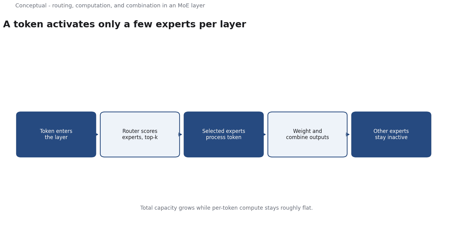
The Switch Transformer paper states the idea clearly: MoE "selects different parameters for each incoming example", producing "a sparsely-activated model — with outrageous numbers of parameters — but a constant computational cost". That is the core trade: total capacity grows while per-token compute stays roughly flat.
Why the economics changed
A dense model's inference cost per token scales with its parameter count. If you double the parameters, you roughly double the arithmetic. An MoE model breaks that link: activating 37B of 671B parameters means the per-token arithmetic resembles a 37B dense model even though the model's total capacity is far larger.
Three consequences follow:
- More knowledge per unit of compute. The model can store more information without paying for all of it on every token.
- Training can be cheaper at a given capacity. Switch Transformers were proposed explicitly to scale "to trillion parameter models with simple and efficient sparsity".
- Quality does not come free. The router must learn to send the right tokens to the right experts, and load imbalance can leave some experts underused.
DeepSeek-V3's technical report describes two specific design choices for these problems: "an auxiliary-loss-free strategy for load balancing" and "a multi-token prediction training objective". The details matter less here than the fact that routing and balance are first-class engineering problems in MoE systems.
A worked example of active parameters
The following uses the published figure from DeepSeek-V3 and hypothetical serving assumptions.
DeepSeek-V3 has 671B total parameters and activates 37B per token. The ratio is:
671 / 37 ≈ 18.1
If inference arithmetic scaled linearly with active parameters, serving this model would cost roughly what a 37B dense model costs per token, rather than what a 671B dense model would cost — about 18× less arithmetic than the dense equivalent.
Three caveats decide whether that saving is real:
- Memory does not shrink. All 671B parameters must be resident somewhere. A model that cannot fit in a single accelerator's memory needs sharding across devices, which adds communication. The Switch paper's "communication costs" are exactly this.
- Routing is not free. The router computation, expert dispatch, and combining outputs add overhead. At short sequences or small batches, that overhead can dominate the arithmetic saving.
- Load balance affects throughput. If one expert receives most tokens, it becomes a bottleneck while others idle. The auxiliary-loss-free strategy exists because naive routing produces this failure.
A practical estimate therefore needs three numbers, not one: active parameters, total memory footprint, and the distribution of tokens across experts.
A model that is cheap in FLOPs but expensive in memory bandwidth is not automatically cheap to serve.
Load balance is an operational metric
In a dense model, every parameter is used on every token, so utilisation is predictable. In an MoE model, the router decides which experts work, and that decision can become uneven. Three symptoms are worth monitoring:
Expert skew. If one expert receives a disproportionate share of tokens, it becomes a bottleneck while other experts sit idle. Throughput falls even though total capacity exists.
Undertrained experts. An expert that rarely receives tokens during training does not learn useful behaviour, so routing to it later produces poor output. This is a training-time problem with deployment-time consequences.
Routing oscillation. Small changes in input can send similar tokens to different experts, which makes behaviour harder to reproduce and debug. A fixed evaluation set is the way to detect it.
DeepSeek-V3's "auxiliary-loss-free strategy for load balancing" is a specific answer to the first two problems. The general lesson is that an MoE system needs utilisation statistics per expert, not only aggregate latency and accuracy. A model can look healthy on aggregate metrics while a single expert is doing most of the work.
Where MoE is the wrong choice
Low-memory environments. If the full parameter set cannot be held, the model may not be deployable at all, regardless of active parameter count. Edge devices are a poor fit.
Very small models. At a small scale, the routing machinery costs more than the experts save. Sparsity pays off when the model is large.
Teams without distributed-systems capacity. MoE training and serving often require sharding, expert parallelism, and careful batching. The complexity that Switch Transformers set out to reduce is still greater than a dense model's.
The counterargument — that dense models are simpler and now cheap enough — is fair for many applications. The reason MoE persists is that the largest models benefit most, and the companies building them have the infrastructure to manage the complexity.
What the papers do not settle
Routing quality is task-dependent. An expert specialisation that helps on one data distribution may not transfer to another. Published evaluations describe the authors' test sets, not yours.
Sparsity is not interpretability. Different experts being active does not mean each expert has a clean human-readable role. Do not read a routing decision as an explanation.
The cost accounting is incomplete. Active-parameter counts describe arithmetic. They do not include memory, network, or the engineering time to keep a distributed serving stack healthy.
A decision test
- Separate total from active parameters in any MoE claim.
- Check the memory footprint — can the whole model be held, or is sharding required?
- Estimate routing and communication overhead, not just FLOPs.
- Ask how load balance is handled and what happens when it fails.
- Compare against a dense model of similar active parameters on your evaluation set.
- Account for the serving team's capability before choosing a distributed architecture.
- Treat expert activation as a mechanism, not an explanation of the model's answer.
For the current model lineups, see LLM Model Landscape 2026; for the infrastructure cost, see Why GPU Computing Is Becoming a Strategic Resource.
References & Further Reading
- Albert Q. Jiang et al., 2024. Mixtral of Experts — Mixtral 8x7B as a sparse mixture of experts, with a router selecting two experts per token at each layer.
- William Fedus, Barret Zoph, Noam Shazeer, 2021. Switch Transformers: Scaling to Trillion Parameter Models with Simple and Efficient Sparsity — The sparsely-activated model argument: huge parameter counts at roughly constant compute, and the barriers of complexity, communication cost and training instability.
- DeepSeek-AI, 2024. DeepSeek-V3 Technical Report — DeepSeek-V3 with 671B total and 37B activated parameters per token, and its load-balancing and multi-token prediction choices.