On this page
- Abstract
- 1. Introduction
- 2. Conceptual Framework: Timing Is a Variable
- 3. Data, Provenance, and Source Integrity
- 3.1 Release dating as a leakage control
- 3.2 Conflicting price feeds
- 4. Feature Engineering and Leakage Control
- 5. Modelling Architecture
- 6. Evaluation Protocol
- 7. Results
- 7.1 Information curve
- 7.2 Main results table
- 7.3 The plot twist: the machine vs one line of code
- 7.4 Walk-forward and holdout
- 7.5 Ablation
- 8. Discussion: What the Model Actually Predicts
- 9. Two Additional Models: Negative Results Reported Anyway
- 9.1 Price-range model
- 9.2 12-month path forecast
- 10. Product Layer
- 11. Threats to Validity and Limitations
- 12. Reproducibility
- 13. Conclusion
- Methodological references
02 / Work
Predicting Monthly Bitcoin Close Direction with Walk-Forward Stacking, Analytic Month-to-Date Rules, and Conformal Quantile Regression: A Comparative Evaluation Against Naive Baselines over 133 Out-of-Sample Months
A walk-forward case study on monthly Bitcoin direction: 133 test months, leakage-controlled features, seven models, a one-line analytic rule, conformal prediction, and a RAG agent —and why the 92% figure is not tradable.
Abstract
This study builds and evaluates a machine learning pipeline for classifying the direction of Bitcoin's monthly close (GREEN or RED) under a strict walk-forward protocol. Data from four external providers —Returnsview, Bitstamp, BLS, and Yahoo Finance— are joined with 71 hand-curated events into daily and monthly panels of 144–155 features. Seven candidate models are evaluated on 133 out-of-sample months after a two-feed price alignment step discards three months with conflicting signs. The GREEN fraction is examined across six information sets, from the previous month-end close (MS) to day 27 of the target month (D27), with a look-ahead audit at end-of-month (EOM).
The main finding is negative, and that negativity is the contribution. At D25 the model reaches 92.5% accuracy and 0.980 ROC-AUC, but a deterministic, zero-parameter rule sign(mtd_ret) reaches 94.0% —a gap of −1.5 percentage points. Every model-versus-rule comparison has a Holm-adjusted p-value of 1.0; the 12-month frozen final holdout yields 91.7% accuracy with an edge of 0.0. Ablation shows that removing the month-to-date block costs 5.3 pp, while removing event features actually improves accuracy. A conformal quantile-regression price-range model loses to a conformally calibrated Gaussian baseline at both published cut-offs, and a 12-month path forecast returns directional accuracy of 30–65% with probability bias of −0.32…+0.01 pp.
The conclusion is that 92% is P(GREEN | move so far this month) —a descriptive quantity that rises because most of the month has already happened by the time the forecast is made— not a signal executable at the prior month-end price. The study deliberately makes no economic claim: no PnL, Sharpe, slippage, or transaction costs are computed. Its value lies in evaluation discipline, leakage control, comparison against an honest baseline, and the reporting of negative results.
Contributions. (i) A formalization of the information set as the variable that determines what "accuracy" means in monthly forecasting; (ii) a walk-forward protocol with inner selection, a skill guard, an analytic champion, and a frozen holdout; (iii) paired statistical testing with multiple-testing correction; (iv) a full reproduction package including a 193-check consistency audit and a RAG agent for automated narrative.
1. Introduction
In popular accounts, forecasting models are often judged by a single accuracy figure. A high number is read as evidence that the model "can predict the market". Two errors are embedded in that reading. First, accuracy is meaningless without stating when the prediction was made: the information available at the start of a month and on day 25 are fundamentally different. Second, accuracy is not the same as a tradable edge; establishing that requires an economic evaluation that accounts for execution price, costs, and capacity.
This study begins with a failure. The first version was a single XGBoost model with an expanding window: 55.7% accuracy, equal to the "always predict GREEN" baseline of 57.1%, and 0.392 ROC-AUC. There was no signal. Instead of changing architectures, the author changed the question asked of the data.
The research questions are:
- RQ1. How much does monthly directional forecast accuracy depend on when the prediction is made, relative to model complexity?
- RQ2. Does a learned model deliver a statistically significant improvement over a deterministic baseline that uses only the sign of the month-to-date move?
- RQ3. Are positive results on directional classification consistent with price-distribution modelling and 12-month path forecasting, or do those tasks reveal the same limitation?
The author writes as a web developer transitioning into data science, so the design emphasizes the details often skipped when the focus is only on modelling: target definition, macro release dating, and consistency between experiment artifacts and the written report. Every number in this article is read directly from the outputs/ directory on 18 November 2026 and can be re-verified with the procedure in Section 12.
2. Conceptual Framework: Timing Is a Variable
Let C_t be the month-end close of month t, and define the monthly label as:
y_t = 1   if  C_t > C_{t-1}        (GREEN)
y_t = 0   if  C_t < C_{t-1}        (RED)
y_t = undefined  if  C_t = C_{t-1} (unlabelled)
The definition is simple, but it forces a decision about when y_t may be known. The study introduces information sets F_d —the information permitted at the moment the forecast for month t is made:
| Set | Forecast moment | Information permitted |
|---|---|---|
MS | Close of month t-1 | Completed months only |
D10, D13, D20, D25, D27 | Day d of month t | MS + month-to-date price movement through day d |
EOM | End of month t | Lookahead — audit only, not a forecast |
This changes the meaning of the metric. Accuracy at MS is a genuine forecast: no information from the target month is used. Accuracy at D25 is an estimate of P(GREEN | information through day 25). Accuracy at EOM is not forecasting at all —it uses the outcome— and is included only to test whether a model "wins" because of information leakage.
Formally, the same model is trained and evaluated for each F_d; the only change is which feature block is admitted. Differences in accuracy across sets can therefore be attributed to when the question is asked, not to the algorithm.
Core insight: "accuracy" cannot be separated from timing. Asking on day 25 is very different from asking at the start of the month —and both differ from seeing the future.
3. Data, Provenance, and Source Integrity
Four providers are combined, plus one manually curated event calendar.
| Data | Source | Role | Notes |
|---|---|---|---|
| Monthly BTC return & close | Returnsview API | Label | The in-progress month is never used as a label |
| Daily BTC OHLCV | Bitstamp via GitHub mirror | Features | mtd_ret, mtd_z_remaining |
| US macro: CPI, core CPI, PPI, NFP, unemployment, AHE | BLS API v2 | Features | Release dating: CPI +15d, PPI +16d, payroll +7d |
| 19 cross-asset series | Yahoo Finance | Features | S&P 500, Nasdaq, VIX, DXY, gold, oil, yields, ETH, COIN, MSTR, etc. |
| Event calendar | Hand-curated, 71 events (2010–2025-06) | Features | Only "days since" / "count in trailing window" |
All data is downloaded once into data/raw/; the pipeline can be re-run with --offline. Provenance is recorded in a registry mapping each column to its source and retrieval time.
3.1 Release dating as a leakage control
BLS macro data is an example of leakage that is invisible unless you look for it: the CPI figure for month t is released roughly 15 days after that month ends. If the CPI value for month t is used to predict y_t at MS or D10, the model sees information that did not exist at prediction time. The study applies release dating: every macro series is shifted to its release date, so a forecast on day d may only use releases that had already occurred. This is a data decision, not a hyperparameter.
3.2 Conflicting price feeds
Labels come from Returnsview while the month-to-date features come from Bitstamp. These are independent sources and they do not always agree:
- median return difference: 0.17 pp;
- maximum difference: 18.6 pp during 2011–2013;
- 3 months disagree in sign —GREEN in one feed, RED in the other.
Those three months are dropped (outputs/source_alignment.json). From 196 available months after alignment, 133 test months remain. The decision shrinks the sample but prevents the model from learning labels that contradict the features used to predict them.
4. Feature Engineering and Leakage Control
Each panel carries 144–155 features, grouped as follows:
- Momentum, volatility, drawdown, RSI across multiple windows;
- Cross-asset returns from 19 Yahoo Finance series;
- Macro features after release dating;
- Event features from 71 curated events;
- Calendar features (seasonality, day of month, etc.);
- Lagged monthly returns;
- Month-to-date block recomputed for each
F_d.
The month-to-date block is the core of the timing experiment:
mtd_ret(d)      = (close_d / close_{t-1}^{EOM} - 1) * 100
sigma_rem(d)    = vol_20d / sqrt(365) * sqrt(H - d)
mtd_z(d)        = mtd_ret(d) / sigma_rem(d)
p_normal(d)     = Phi(mtd_z(d))
where H is the number of days in the month and Phi is the standard normal CDF. p_normal(d) is the "normal-model P(GREEN)" under the assumption that the remaining move is directionless. It serves as the analytic champion that competes with the learned models (Section 5).
Pipeline discipline. Scaling, imputation, and feature selection live inside a scikit-learn Pipeline and are fitted only on the training window. No transformer ever sees test data. This enforces leakage control structurally: correctness does not depend on the researcher remembering a rule during an experiment.
Ablation is then used to test which feature block actually contributes (Section 7.5).
5. Modelling Architecture
Candidate models span linear models, trees, and rule-based models:
| # | Component | Role |
|---|---|---|
| 1 | LogisticRegression L1/L2 | Linear baseline |
| 2 | RandomForest, ExtraTrees | Tree ensembles |
| 3 | XGBoost, LightGBM | Gradient boosting, deliberately shallow/regularized |
| 4 | rule_logreg, rule_controls_logreg | Analytic anchors (3 features) |
| 5 | Phi(mtd_z) | Analytic champion, 0 parameters, untrained |
Selection flow:
sources → daily panel → monthly panel → walk-forward
        → inner expanding validation → skill guard → champion
        → forecast → dashboard / agent
Inner expanding validation. Inside each training window, chronological inner validation selects stacking weights, the decision threshold, and a meta-learner (logistic regression on member logits). Inner validation never touches test data.
Skill guard. The model is forbidden from emitting a signal unless it beats the majority prediction and its inner-validation ROC-AUC is at least 0.53. This prevents spurious signals from models that are not statistically better than a guess.
Analytic champion. The Phi(mtd_z) rule competes on a chronological holdout. Stacking is used only if it beats the rule; ties are awarded to the analytic rule. The default is conservative: complexity must pay for itself.
Frozen final holdout. The last 12 months are never used to select a model, threshold, or configuration. The holdout is opened once at the end (outputs/final_holdout.json).
6. Evaluation Protocol
The protocol is designed to answer RQ2 with defensible statistics.
- Split: 60 initial training months followed by expanding walk-forward; 133 out-of-sample months.
- Metrics: directional accuracy and ROC-AUC per information set.
- Paired test: McNemar's test for differences in paired proportions (model vs sign rule).
- Multiple-testing correction: Holm's procedure applied across all comparisons. Without it, one fortuitous significant comparison would look like a finding.
- Diebold–Mariano test: an additional check for comparative predictive accuracy.
- Ablation: one feature block removed at a time to locate the source of signal.
- Holdout: the last 12 months opened once, after all design decisions are frozen.
The study deliberately does not compute PnL, Sharpe ratio, slippage, or transaction costs. Consequently, no economic edge can be claimed from these results —and none is claimed.
7. Results
7.1 Information curve
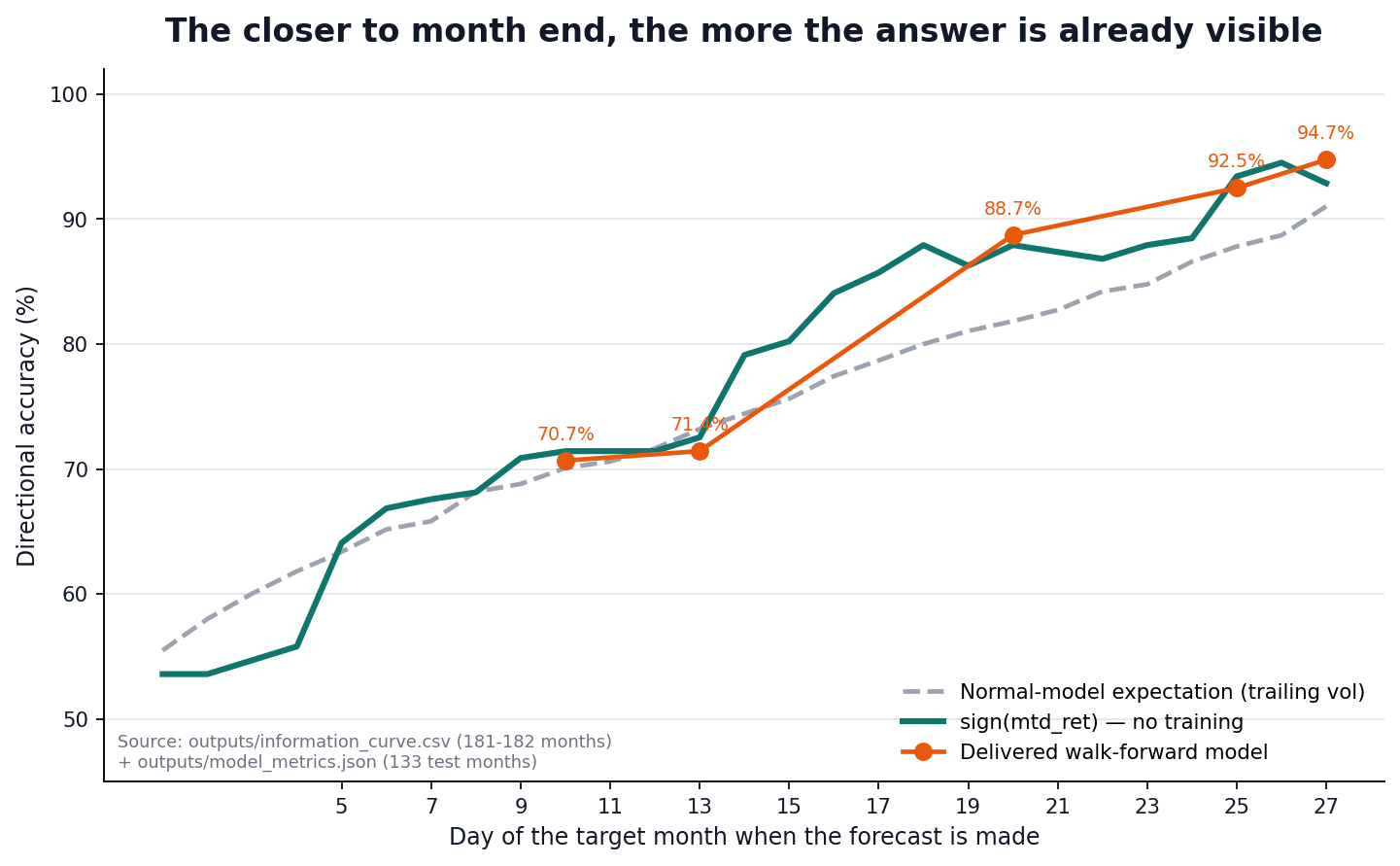
Figure 1. Accuracy as a function of forecast day. The dashed line is the normal-model expectation, the green line the untrained sign rule, and the orange points the delivered walk-forward model. Source: full-resolution figure ↗ · data: outputs/information_curve.csv and outputs/model_metrics.json.

The curve shows the pattern that dominates every experiment: accuracy rises as month end approaches. Model, sign rule, and normal expectation all move in the same direction. Added complexity does not change the shape of the curve.
7.2 Main results table
The following summary must be read as a whole —including the edge and p-value columns:
133 out-of-sample months · 60 initial training months · expanding walk-forward

Set     Model   sign(mtd_ret)   Edge       AUC     p_Holm
MS      45.9%   n/a             n/a        0.418   n/a
D10     70.7%   72.2%           -1.5 pp    0.776   1.0
D13     71.4%   72.2%           -0.8 pp    0.784   1.0
D20     88.7%   88.0%           +0.8 pp    0.932   1.0
D25     92.5%   94.0%           -1.5 pp    0.980   1.0
D27     94.7%   94.0%           +0.8 pp    0.981   1.0
EOM*    93.2%   —               —          0.991   —
(* lookahead audit, not a forecast)
Two facts stand out. First, the model's edge over the sign rule ranges from −1.5 to +0.8 pp —smaller than the sampling uncertainty. Second, every Holm-adjusted p-value is 1.0: after accounting for the number of configurations tried, not a single difference is significant.
7.3 The plot twist: the machine vs one line of code
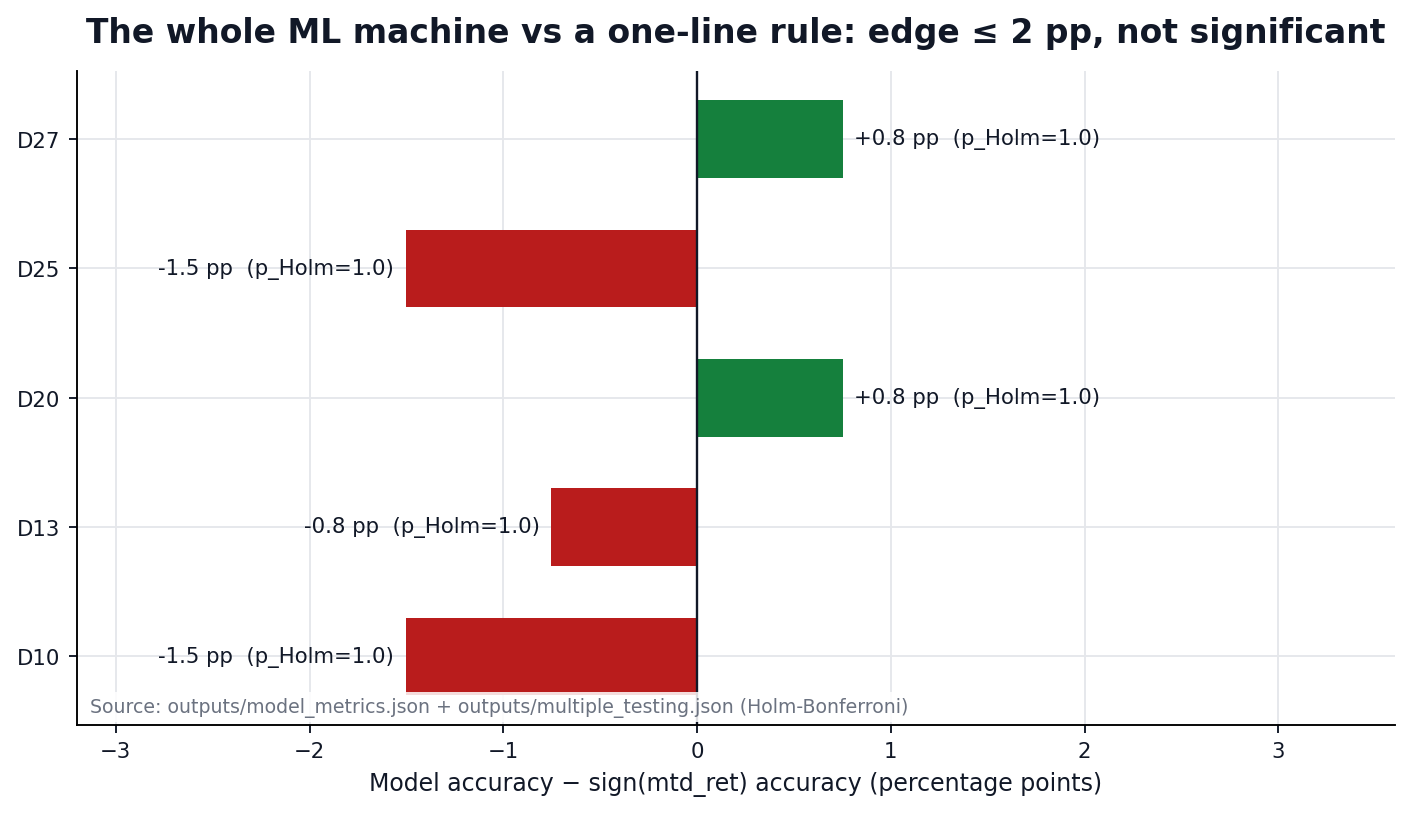
Figure 2. The entire ML machine versus a one-line rule. Each bar is an accuracy difference in percentage points; no bar is significant after Holm correction. Source: full-resolution figure ↗ · data: outputs/model_metrics.json and outputs/multiple_testing.json.

At D25 the model reaches 92.5% while sign(mtd_ret) reaches 94.0% —the model loses by 1.5 pp to a rule with no parameters that requires no training. The most compact statement of this result:
The most accurate part of the model was the part that needed no training at all.
7.4 Walk-forward and holdout
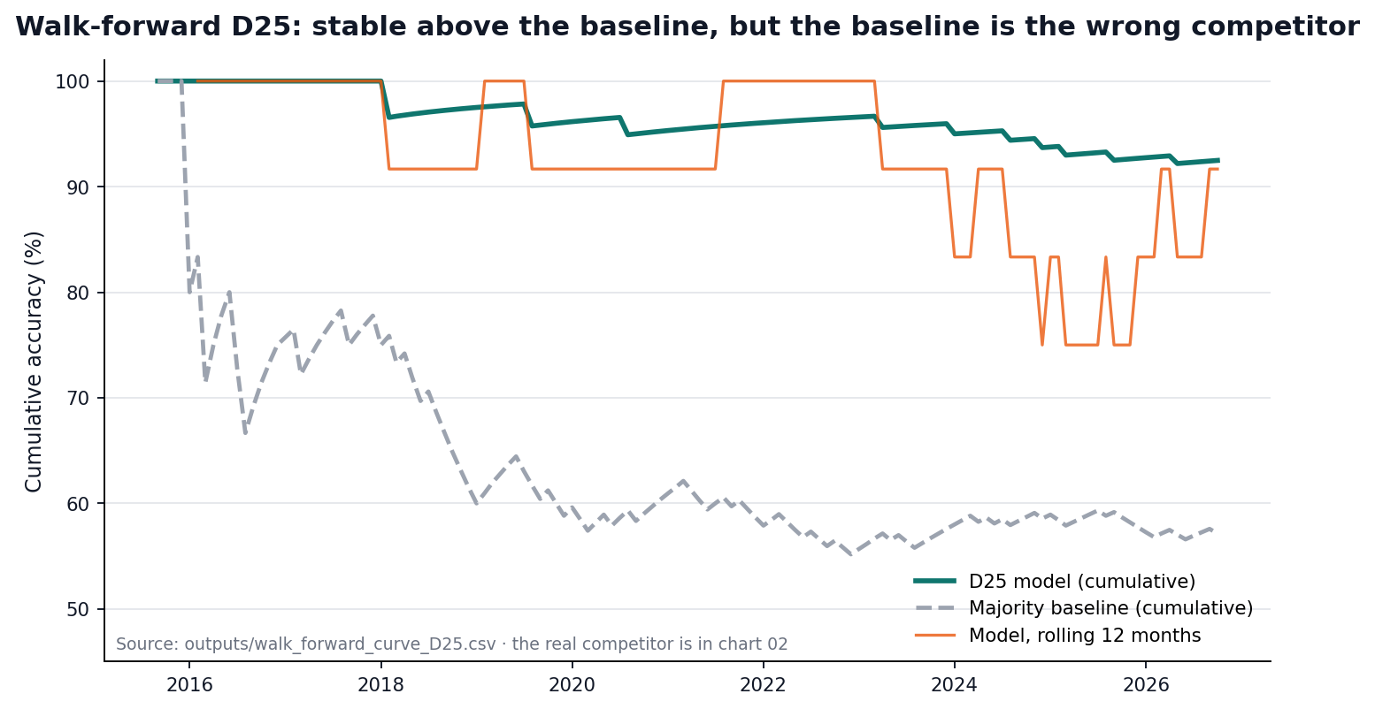
Figure 3. Cumulative D25 accuracy against the majority baseline. The model looks stable above the baseline, but the majority baseline is not the right competitor; the right competitor is in Figure 2. Source: full-resolution figure ↗ · data: outputs/walk_forward_curve_D25.csv.

The cumulative curve is a common methodological trap. Relative to "always predict GREEN", the model looks far better. Relative to the sign rule, the advantage disappears. The frozen 12-month holdout gives 91.7% accuracy with an edge of 0.0 over the sign rule —model selection produces no advantage that survives on unseen data.
7.5 Ablation
The D25 ablation tests which feature block actually works:
| Configuration | Accuracy |
|---|---|
| Full | 92.48% |
| Without events | 93.99% |
| Without macro | 92.48% |
| Without month-to-date | 87.22% |
Removing events raises accuracy by 1.51 pp, so the claim that macro or calendar features improve performance is unsupported. Removing the month-to-date block lowers accuracy by 5.26 pp. The conclusion is narrow and clear: only the month-to-date signal works, and that signal is available without a model.
8. Discussion: What the Model Actually Predicts
By day 25, the month's move is nearly final and already known to every market participant. The 92.5% figure is therefore not a forecast of the future; it is the descriptive statement P(GREEN | move so far this month). The EOM audit, which deliberately lets the model peek at the final outcome, yields 93.2% —no more convincing than the honest D27 set at 94.7%. If peeking at the answer adds no confidence, the high accuracy comes from information already visible, not from a hidden pattern the model uncovered.
The practical consequence: this score cannot be executed at the previous month-end price. Turning it into an edge would require evaluation against real execution prices, slippage, costs, and capacity. None of that exists in this study.
92% accuracy at day 25 does not mean we can predict Bitcoin. It means most of the month has already happened by day 25.
The author deliberately does not paper over this. Selling 92% as "the model predicts Bitcoin" makes a better story —and a false one.
9. Two Additional Models: Negative Results Reported Anyway
To test whether the directional finding is task-specific or a symptom of a broader signal limit, two further models were built.
9.1 Price-range model
The price distribution model uses LightGBM quantile regression at the 5/10/25/50/75/90/95% levels, with conformal calibration (Romano et al., 2019). It is compared against a Gaussian band calibrated conformally in the same way. The metric is CRPS (continuous ranked probability score), where lower is better.
| Cut-off | Model CRPS | Naive band CRPS | Winner |
|---|---|---|---|
| D13 | 8.547 | 8.204 | naive |
| D25 | 3.542 | 3.481 | naive |
The learned model loses at both published timings, so the deployed baseline is the Gaussian band. An older version of the README showed only the timing where the model won; that has been corrected. Selective reporting of this kind is cherry-picking and has no place in a case study.
9.2 12-month path forecast
The path model uses 300 Monte Carlo paths with a 30-day block bootstrap of log returns, with de-meaning performed after volatility scaling. Macro features are carried forward. The backtest uses 24 origins, with refitting before each origin —without refitting, the evaluation would optimistically use parameters that had already seen the future.
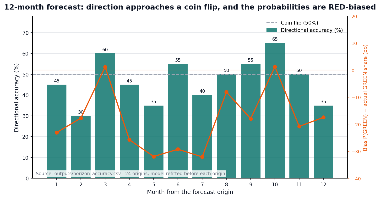
Figure 4. Directional accuracy by month from origin (left) and probability bias against the actual GREEN share (right). Source: full-resolution figure ↗ · data: outputs/horizon_accuracy.csv, 24 origins, model refitted before each origin.

Directional accuracy ranges from 30% to 65% —close to a coin flip— with probability_bias of −0.32…+0.01 pp. The probabilities are not used; only the price ranges are useful. This is consistent with RQ3: the same limitation reappears when the question changes from "direction this month" to "the path over 12 months".
10. Product Layer
Three product layers keep the research from ending in a notebook.
BI dashboard. FastAPI + Plotly.js, seven pages, a star-schema cube with cross-filtering, URL state, PNG/CSV export, vendored Plotly for offline use, light/dark themes, and a STALE DATA badge when data or the cut-off is old.
Research agent. LangGraph + RAG combining BM25 and TF-IDF with reciprocal rank fusion over project artifacts. An OpenAI-compatible LLM with an offline fallback, SQLite checkpoints, a run registry, and a number_audit module that verifies every percentage in a memo against retrieved context.
Audit script. 193 checks ensure numbers in the dashboard and reports still match the pipeline files. The point to emphasize: the audit guarantees consistency, not method validity. It answers "does the article match the outputs?", not "is the method correct?". Keeping these separate prevents a helper tool from being mistaken for scientific evidence.
I built an audit that proves my dashboard is consistent. It cannot prove my method is right — that is a different, harder question.
Final status: 193 checks, 0 failed; tests 55 passed, 1 skipped.
11. Threats to Validity and Limitations
The limitations must be stated alongside the results:
- Small sample. 133 out-of-sample months for a single asset; confidence intervals are wide and generalization to other assets is untested.
- Post-hoc protocol. Some exploration preceded the final protocol; this weakens statistical inference even though the holdout was frozen.
- No vintage data. BLS macro values are final/revised figures, not the values available at the historical release date. Release dating fixes availability in time, not later revisions.
- No economic evaluation. No PnL, Sharpe, costs, or capacity —so no claim of tradability.
- Late-month accuracy is descriptive. Figures at D25/D27 are
P(GREEN | move so far), not a signal executable at the prior month's close. - Not financial advice. All results are research experiments, not investment recommendations.
Translated, these limitations mean the study is worth presenting as an exercise in research discipline, not as a production-ready prediction system.
12. Reproducibility
Code structure and reproduction procedure:
btcml/
  config.py        constants, data universe, event calendar, holdout
  sources.py       downloader + cache + stale warnings
  features.py      daily panel → monthly panel, two-feed alignment
  models.py        candidate models + rule-anchored models
  walkforward.py   engine, champion, skill guard, metrics, DM test, Holm
  analysis.py      benchmark, ablation, information curve
  forecast.py      Monte Carlo path + backtest refit-per-origin
  range.py / range_runner.py   quantile + conformal price range
  provenance.py    data-source registry
  dashboard/       FastAPI + Plotly + star-schema cube
  agent/           LangGraph + RAG + number audit
  scripts/
    make_portfolio_charts.py     article figures
    make_ci_fixture.py           deterministic synthetic data for CI
    audit_console.py             193 consistency checks
Full reproduction:
pip install -e ".[dev,agent]"
python train_btc_monthly.py --offline --sets MS,D10,D13,D20,D25,D27 --live-day 13 --no-ranges
python train_btc_monthly.py --offline --ranges-only --live-day 13
python scripts/make_portfolio_charts.py
python scripts/audit_console.py          # must be 0 failed
PYTHONPATH=. python -m pytest tests/     # 55 passed, 1 skipped
Article figure catalogue (all generated from outputs/):
| File | Content |
|---|---|
portfolio_01_information_curve_en.png | Accuracy vs forecast day |
portfolio_02_edge_vs_sign_rule_en.png | Edge + p_Holm (Figure 2) |
portfolio_03_walkforward_curve_en.png | Cumulative D25 accuracy |
portfolio_04_horizon_bias_en.png | 12-month accuracy + bias |
The live dashboard and research agent are deployed at btc-monthly-close-prediction.vercel.app. The source code is available as a public repository: novanr511/btc-monthly-close-prediction. It includes the walk-forward engine, dashboard, RAG agent, offline fixture, and the 193-check audit script, so every number in this article can be reproduced from the pipeline outputs.
13. Conclusion
Five lessons from this study:
- An honest baseline saves the narrative. Without the
sign(mtd_ret)rule, 92.5% reads as success. With it, the same number reads as evidence that most of the month had already happened. - Feature engineering beats model complexity. The month-to-date block contributes 5.3 pp; the entire stacking machine contributes an edge of at most 2 pp, statistically insignificant.
- An audit of consistency is not validity. 193 checks keep the numbers in sync; they do not prove the method right.
- Negative results are publishable. The quantile model lost and the path forecast approached a coin flip —both are recorded, not hidden.
- A dashboard and an agent make research consumable. Research that lives only in a notebook cannot be examined by readers; the product layers make it inspectable.
The most accurate part of the model was the part that needed no training at all.
The value of this project is not its 92% accuracy, but the process that proved 92% is not a tradable edge —and the decision to say so plainly.
Methodological references
The methods used follow the literature below. This list references methods, not claims of novelty:
- Diebold, F. X. & Mariano, R. S. (1995). Comparing predictive accuracy. Journal of Business & Economic Statistics.
- McNemar, Q. (1947). Note on the sampling error of the difference between correlated proportions or percentages. Psychometrika.
- Holm, S. (1979). A simple sequentially rejective multiple test procedure. Scandinavian Journal of Statistics.
- Romano, Y., Correa, J. & Candès, E. J. (2019). Conformalized quantile regression. NeurIPS.
- Pedregosa, F. et al. (2011). Scikit-learn: Machine learning in Python. JMLR —for
Pipelinediscipline in leakage prevention.
Disclaimer: this is a research note, not financial advice. No claim is made that the model can be used for trading, and no evaluation of PnL, costs, or capacity was performed.