Compound Interest Examples That Make It Click
Compounding is return on return. Read three worked examples, the effect of time and fees, and why a constant rate is a teaching device.
Compound interest is easy to define and hard to feel. The formula says that returns earn returns, which means time matters more than most people expect and fees matter more than they appear. A few worked numbers make the mechanism clearer than another explanation of the formula.
Direct answer: Compounding means that each period's return is calculated on the original principal plus previous returns. Investor.gov describes compound growth as earning "a return on money you invest as well as on the return your invested money earns", and uses a 7% average annual rate as an illustration of long-term diversified US stock returns — explicitly as an estimate, not a promise. The boundary: real returns vary, inflation reduces purchasing power, and a constant rate is a teaching device rather than a forecast.
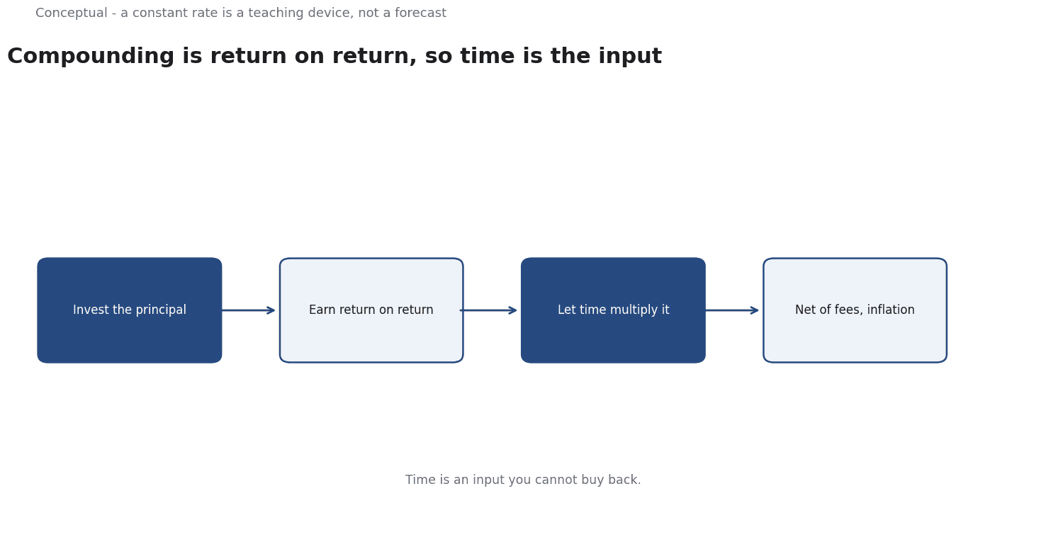
Example one: time matters more than amount
The following numbers are hypothetical and illustrative, using a constant 7% annual return.
- Saver A invests 2,000 a year from age 25 to 35 — ten years, 20,000 total — then stops.
- Saver B invests 2,000 a year from age 35 to 65 — thirty years, 60,000 total.
At age 65, with annual compounding:
- A's balance: roughly 94,000 from 20,000 contributed.
- B's balance: roughly 189,000 from 60,000 contributed.
Three times the contributions produce only twice the balance, because A's money had thirty more years to compound.
The lesson is not that early saving is easy; it is that time is an input you cannot buy back.
Example two: the cost of a fee
A fund returns 7% a year before a 1% annual fee. Over 30 years, the difference between a 7% and a 6% outcome on a 10,000 initial investment is roughly:
- 7% for 30 years: about 76,000.
- 6% for 30 years: about 57,000.
A fee that looks small each year removes about 19,000 of the ending value in this example — a quarter of the gross outcome. The arithmetic is exact under the assumed constant rates; the point about fees holds under variable ones, though the magnitude changes.
This is why cost is a first-order variable in long-term investing, as Personal Finance for Professionals: Managing Income, Saving, and Investing explains.
Example three: nominal versus real
If an investment returns 7% and inflation averages 3%, the real return is approximately 4% — not 7%. Over 30 years, the difference in purchasing power is large:
- Nominal growth of 10,000 at 7%: about 76,000.
- Real growth at 4%: about 32,000.
Three readings follow:
- A goal stated in today's pounds needs a real return. Using a nominal rate to plan a retirement income overstates what that income will buy.
- Inflation is not a suggestion in the model. It is a variable with its own data and uncertainty. FRED publishes dated inflation series that can be used with a stated period.
- Taxes are a fourth adjustment. A return before tax is not the return available to spend, which is why tax-efficient investing is a separate topic.
Why the order of returns matters
A constant rate hides a property that matters in real portfolios: losses and gains arrive in an order, and that order changes the outcome when money is being added or withdrawn. A portfolio that falls 30% in the first year and recovers later needs new contributions to buy more units at low prices, which can improve the final result. A portfolio that rises first and falls later, with withdrawals during the decline, can end lower than a constant-rate calculation suggests.
This is why a single average return is a poor summary of an investment experience. Two decades with the same average can produce different ending balances if the sequence differs. The practical implication is modest but useful: focus on contributions and costs, which you control, and treat the order of returns as uncertainty rather than a variable you can plan around.
The examples above deliberately use a constant rate because the arithmetic is transparent. They are a way to understand the mechanism, not a promise about any particular sequence of years.
What the examples assume
A constant rate. Real returns arrive in an irregular sequence, and the order matters when contributions and withdrawals are involved. A constant rate is a teaching device, not a description of any actual year.
Reinvestment. The calculation assumes returns are reinvested. Taking them as income changes the result.
No taxes. Tax treatment varies by account and jurisdiction, and it changes the effective compounding rate.
No behavioural interruptions.
The modelled result assumes the investor holds, which is a choice, not an automatic consequence of opening an account.
The counterargument — that these caveats make the examples useless — is wrong. They make the examples honest.
The mechanism is real; the numbers are illustrative.
A decision test
- State the goal in real terms if it is far in the future.
- Use a rate with a source and describe it as an estimate.
- Subtract fees before judging the outcome.
- Account for inflation with a stated period.
- Check the tax treatment of the account.
- Treat the result as a range across plausible rates.
- Focus on what you control — contributions, costs, and time in the market — rather than the exact return.
For the account context, see Personal Finance for Professionals; for the inflation data, see FRED.
References & Further Reading
- U.S. Securities and Exchange Commission (Investor.gov), 2026. Introduction to Investing — Primary regulator guidance on market mechanics and investor protection.
- Federal Reserve Bank of St. Louis, 2026. FRED economic data — The primary time-series database used for macro indicators.