Hyperparameter Tuning: Grid Search, Random Search, and Bayesian Optimization
Most hyperparameters do not matter much. Read the evidence on why random search beats grids and when a smarter search pays for itself.
Hyperparameter tuning is often treated as a tedious but mechanical step: list the options, try them all, pick the best. The trouble is that "try them all" is impossible in any realistic space, and the choices about what to try are where most of the value — and most of the waste — sits. The best-known empirical result in this area is that the obvious strategy is usually the wrong one.
Direct answer: Grid search spends compute uniformly across a configured space, which is wasteful when only a few hyperparameters materially affect the result. Bergstra and Bengio found that "random search over the same domain is able to find models that are as good or better within a small fraction of the computation time" than grid search, and that at the same budget it "finds better models by effectively searching a larger, less promising configuration space". Bayesian and bandit-based methods go further by allocating trials adaptively, but they cost more to run and are not automatically better.
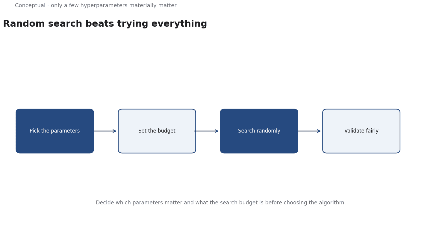
The practical discipline is to decide which parameters matter and what the search budget is before choosing the algorithm.
Why grid search fails
A grid is defined by the user: a list of values for each hyperparameter, and every combination is evaluated. Its effort grows multiplicatively with the number of parameters, so a grid that looks modest on paper becomes enormous quickly — ten values for five parameters is 100,000 configurations.
The deeper problem is that the grid is not a representative sample of the space. If two of the five parameters matter and three do not, the grid spends most of its 100,000 evaluations on combinations that differ only in the irrelevant ones. It explores thoroughly in the directions that do not matter.
Bergstra and Bengio's comparison makes the consequence concrete. Against deep belief networks configured by "a thoughtful combination of manual search and grid search", purely random search over the same 32-dimensional space "found statistically equal performance on four of seven data sets, and superior performance on one of seven". The authors conclude that "this phenomenon makes grid search a poor choice for configuring algorithms for new data sets".
That is a strong claim, and it is bounded: it is a comparison on specific models and datasets, not a theorem that grids are always worse. What generalises is the mechanism — when few parameters matter, uniform enumeration is a bad allocation of trials.
Random search is a baseline, not a shortcut
Random search draws configurations from distributions over each parameter. Its virtue is that it samples broadly in every dimension, so it is more likely to find a good value for the one or two parameters that actually matter, and it goes deeper along those dimensions than a grid of the same size.
Two practical consequences follow. First, the distributions matter more than the algorithm. If a learning rate is sampled uniformly between 0 and 1, almost every draw will be useless; a log-uniform distribution over a sensible range is a better search space and requires no cleverer optimiser. Second, random search is embarrassingly parallel and easy to reproduce, which makes it a strong baseline that more sophisticated methods must beat.
The honest comparison is not "random versus grid" but "what does a well-chosen search space plus random sampling achieve for this budget?"
Adaptive methods and what they buy
Bayesian optimisation builds a model of the objective — how configuration settings relate to performance — and uses it to choose the next trial, balancing exploration of uncertain regions against exploitation of promising ones. It is sample-efficient when evaluations are expensive and the space is not too high-dimensional, and it adds its own hyperparameters and assumptions.
Hyperband takes a different approach. Li et al. formulate tuning as a "pure-exploration non-stochastic infinite-armed bandit problem" in which a resource such as iterations, data samples, or features is allocated to randomly sampled configurations. The method uses "adaptive resource allocation and early-stopping" to speed up random search, and the paper reports that Hyperband "can provide over an order-of-magnitude" improvement in the settings tested. Its insight is cheap and powerful: most configurations are bad, and you can find out with a small budget, so spend the full budget only on the survivors.
Optuna represents a different design choice — define-by-run search spaces, where the configuration is built by the code as it runs rather than declared in a static block. Its documentation describes pruning as a first-class mechanism, which is the same early-stopping idea expressed at the framework level.
AutoML systems extend this to choose models and features as well as hyperparameters. Auto-sklearn's approach combines meta-learning — using performance on similar datasets to pick a starting point — with ensemble construction. It is useful when the cost of human expertise exceeds the cost of compute, and it makes the search harder to interpret.
A worked budget comparison
The choice of search method is easier to see with numbers. Suppose a model has five hyperparameters and a full training run costs ten minutes, with a total budget of 500 runs.
- A grid of four values per parameter costs 4⁵ = 1,024 runs — twice the budget — and varies only four settings per parameter. If two parameters matter and three do not, roughly 96% of the runs duplicate the useful variation across irrelevant dimensions.
- Random search at 500 runs samples 500 distinct five-tuples. For the two parameters that matter, it explores roughly 500 distinct combinations, and it is far more likely to find a good value for both than the grid's 16 useful combinations.
- Hyperband at the same budget might start 5,000 configurations with a tenth of the training budget each, keep the best 500 after early evaluation, and spend the remaining budget on those. The expensive evaluations are concentrated on candidates that survived a cheap test.
The numbers are illustrative, not a benchmark, and that is the point: the comparison can be made before any code is written. A team that knows its per-run cost and its total budget can decide how many trials it can afford and which method uses them best, rather than discovering after a week that the grid will not finish.
The same arithmetic exposes a second problem. Running 500 trials and reporting the best score is a multiple-comparisons problem: with enough trials, a configuration will appear excellent by chance. The score that matters is the one on a nested held-out set, evaluated once, and the gap between the selection score and that final score is a measure of how much the search overfitted the validation set.
The evaluation that makes tuning meaningful
Every tuning method needs a score, and the score is where the whole exercise can be invalidated.
A configuration selected on the test set is no longer a held-out estimate; the test set has become training data. The discipline is a nested split: an outer split for the final estimate and an inner one for choosing configurations. scikit-learn's TimeSeriesSplit adds a further requirement for time-ordered data — expanding folds with a gap where labels arrive late.
Tuning also amplifies leakage. If preprocessing is fitted on the full dataset before the search, every configuration is scored on an optimistic number, and the search will reliably find the configuration that exploits the leak. scikit-learn's guidance that leakage occurs when "information that would not be available at prediction time is used when building the model" applies to every trial, not just the final model.
The practical rule: treat the tuning loop as part of the pipeline, and make the split boundaries impossible to cross.
A budget-first process
- Set the budget in evaluations and wall-clock time before choosing a method. Search complexity without a budget is not a plan.
- Choose sensible distributions for each parameter, using a log scale where the parameter spans orders of magnitude.
- Run random search as the baseline and record its best score and the time taken.
- Add adaptive methods only if the baseline is insufficient, and compare them on the same budget and splits.
- Use early stopping where a configuration can be judged cheaply, as Hyperband does.
- Keep a nested evaluation so the reported score is not the score used to select.
- Check whether the gain is real. A difference that changes with the random seed is noise, and the number of trials needed to establish it is part of the cost.
For the evaluation framework, see MLOps; for the model families being tuned, see Deep Learning Basics.
A worked example
The following is hypothetical and illustrative. A team has a budget of 500 training runs across five parameters and compares two plans. First, a grid of four values per parameter costs 1,024 runs, exceeds the budget, and varies only four settings for each parameter. Second, random search at 500 runs samples distinct five-tuples and, if two parameters carry most of the effect, explores far more useful combinations than the grid's sparse coverage. Third, both plans are evaluated on a held-out split, because tuning without a fixed evaluation rewards noise rather than generalisation. The outcome is bounded: random search is likely to find a better configuration under this budget, but it offers no guarantee of the optimum, and a budget-first process matters more than the choice of sampler. The three checks decide the plan, not the result.
A counterargument
A fair critic would argue that the article promotes a bounded empirical finding into a general rule. Bergstra and Bengio's result is explicitly a comparison on specific deep belief networks and data sets, and Li et al. report Hyperband's order-of-magnitude gain only "in the settings tested", yet the guide turns these into a default that random search is the baseline all other methods must beat. In a low-dimensional space, or where parameters interact strongly, a grid is affordable and exhaustive, and the article's own "illustrative, not a benchmark" example does not establish otherwise. A critic could also say that calling adaptive methods merely "not automatically better" understates the cited evidence: Optuna's pruning and auto-sklearn's meta-learning exist because sample efficiency can matter.
The mechanism is sound; its universality is assumed rather than shown.
References & Further Reading
- James Bergstra and Yoshua Bengio, 2012. Random Search for Hyper-Parameter Optimization — Why random search beats grid search in high-dimensional hyperparameter spaces.
- Liam Li et al., 2017. Hyperband: A Novel Bandit-Based Approach to Hyperparameter Optimization — Successive halving as a way to spend a fixed budget across fidelities.
- Taku Akiba et al., 2019. Optuna documentation — Define-by-run search spaces and pruning strategies, in the documentation of a widely adopted tuner.
- Thomas Ferré et al., 2015. Efficient and Robust Automated Machine Learning — Meta-learning plus ensemble construction, and the real cost of automated tuning.