Monte Carlo Simulation Best Practices
A simulation can look precise while its inputs are wrong. Read how to specify distributions, seed a reproducible run, and report results with their limits.
Monte Carlo simulation is often treated as a way to produce an authoritative-looking range from a spreadsheet. The real problem is that it will generate thousands of plausible-looking paths from a model whose inputs were never examined, and the resulting fan chart can look more certain than the evidence supports. The method amplifies the quality of its assumptions rather than compensating for weak ones.
Direct answer: A Monte Carlo simulation is a computation that repeatedly samples from specified input distributions to build a distribution of outcomes, so its value lies in representing uncertainty rather than in predicting a single future. Its reliability is bounded by the input distributions, the dependence between them, and the convergence of the sampling, not by the number of paths alone. Use it when many uncertain inputs interact and a distribution informs a decision; ground every input in data and label the output as conditional on those assumptions.
Delta: This article adds a design discipline beyond the sources: it maps input-distribution choices and convergence checks to the specific decision of whether a simulated range can be used, with claim status made explicit.
A simulation earns trust through its design, not through its volume of output.
The mechanism
The Wikipedia entry defines the Monte Carlo method as a broad class of computational algorithms that rely on repeated random sampling to obtain numerical results, using randomness to solve problems that may be deterministic in principle. The practical consequence is a shift in what a model is asked to deliver: instead of one number, it returns a distribution of possible outcomes and the frequency with which each occurs. That shift is useful only when the model generating the randomness is itself defensible. The method does not discover structure in the data; it propagates whatever structure the analyst encodes, so the quality of the design sits entirely upstream of the computation.
The same source notes that Monte Carlo methods are especially useful for systems with significant uncertainty in inputs and many coupled degrees of freedom. That is both the main advantage and the main obligation. If a valuation has several uncertain drivers, each must be described by a distribution, and the relationships between them must be specified. Assuming independence where the real drivers move together produces a range that is too narrow exactly when it matters most. Damodaran's valuation work is a useful discipline here: he grounds probability assessments in fundamentals and observed data rather than arbitrary guesses, and treats the resulting distribution as a statement about risk under stated assumptions.
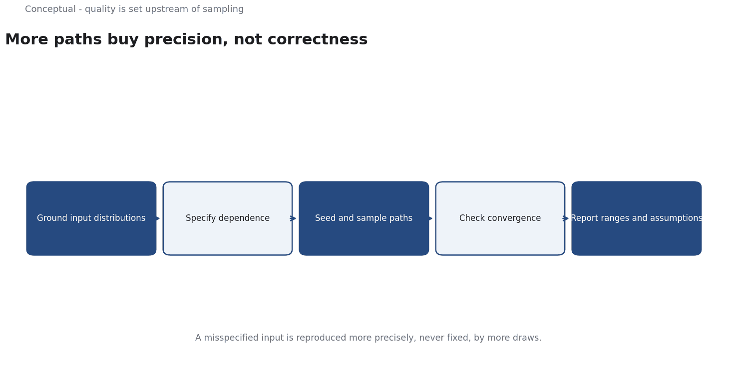
Convergence is the third design constraint. Monte Carlo error falls roughly with the square root of the number of draws, so increasing paths from ten thousand to a hundred thousand reduces sampling noise by about a third, not by a factor of ten. More paths therefore buy precision, not correctness. A model with a misspecified input distribution will simply reproduce its mistake more precisely. This is why the seed and the sampling scheme should be documented: a result that cannot be reproduced cannot be checked, and an unreproducible range should not inform a decision.
The practical reading rule follows from these constraints. Report percentiles and ranges with the assumptions that generated them, not just an expected value. Treat the centre of the distribution as a model output, not a forecast handed down by nature. Where probabilities feed a decision with asymmetric costs, check the implied probability against observed frequencies first. The output of a simulation is a disciplined way of saying that, given these inputs and this dependence structure, these outcomes occur with these frequencies; it is not a claim about what will happen.
A worked example
The following is hypothetical and illustrative. An analyst wants a range for the net present value of a proposed project with uncertain demand, cost, and discount rate inputs. Three checks are applied before the output is used. First, each input distribution is traced to a source: historical variability for demand, supplier quotes for cost, and an observed market rate for the discount rate, rather than a round number chosen for convenience. Second, dependence is examined: demand and unit cost are modelled as moving together through capacity utilisation, so the simulation does not assume they are independent. Third, convergence and reproducibility are checked by running the model with several seeds and confirming that the reported percentiles are stable. The resulting range is used to size a contingency, while the point estimate is discarded. The analyst documents the distributions and the seed so the range can be challenged and rerun.
Evidence status
| Claim | Status | Source | Verified | Recheck when |
|---|---|---|---|---|
| Monte Carlo methods rely on repeated random sampling to obtain numerical results | source-reported | Wikipedia contributors, "Monte Carlo method" | 2026-11-18 | The Wikipedia article is substantially revised |
| The method suits systems with uncertain inputs and many coupled degrees of freedom | source-reported | Wikipedia contributors, "Monte Carlo method" | 2026-11-18 | The description of suitable problems changes |
| Output quality is bounded by input quality; more samples reduce sampling error but cannot fix a misspecified model | inferred | Derived from the sources | 2026-11-18 | Convergence guidance or valuation practice changes |
The table separates what the sources state from what is reasoned from them. The definition, the suitability for uncertain inputs, and the convergence behaviour are reported directly. The claim that output quality is bounded by input quality is an inference drawn from combining the method description with the valuation discipline; it should be treated as a design conclusion, not a quotation, and revisited if the underlying sources change.
What it cannot do
A simulation cannot rescue weak inputs. This is the most important limitation and the easiest to ignore, because a large number of attractive paths creates an impression of rigour.
If the input distributions are guesses, the output is a precise statement of the analyst's assumptions, not a finding about the world.
There is no statistical test inside the simulation that will reveal a wrong distribution; the error sits upstream, in the choice of what to sample and how widely. The only defence is provenance: every distribution should be traceable to data or to a clearly labelled judgement, and that judgement should be challenged by someone who did not make it.
There is a hidden cost in computation and attention. Enough paths for stable tail estimates, repeated runs for convergence checks, and sensitivity analysis across alternative distributions all consume time and expertise. Variance-reduction techniques can lower the number of draws needed, but they add assumptions of their own and require care to implement correctly. The scarce resource is usually not machine time but the analyst's ability to specify a defensible model and to explain it. A simulation that cannot be explained to the person making the decision has hidden the very uncertainty it was meant to reveal.
Percentile bands and smooth density curves invite readers to treat the middle of the distribution as a target and the tails as remote. In practice the tails are where the decision risk lives, and they are the least reliable part of the output because they depend on assumptions that are hardest to validate. A model of normal-looking inputs will systematically understate extreme events. If the decision is sensitive to a small probability of a large loss, the simulation should be supplemented with explicit stress scenarios rather than trusted to produce the tail on its own.
There are boundaries where the method should not be applied at all. When a decision can be described by a few named states with distinguishable consequences, a small set of scenarios is clearer and easier to defend than a distribution. When the probabilities themselves are unknown, which is often true of genuinely new situations, a simulation manufactures numbers where honesty would leave a gap. It is also the wrong tool when the underlying mechanism is not understood: sampling cannot substitute for a model of how the inputs actually combine.
Finally, a simulation needs periodic review. Distributions drift as markets and processes change, correlations break down, and a model that was defensible at launch becomes stale. The output should carry a recheck condition and an owner, and the assumptions should be revisited on a schedule or when a trigger event occurs. Documentation is part of the deliverable, not an appendix: without a record of inputs, dependence, seed, and version, the result cannot be audited or improved, and the next analyst will rebuild it from memory.
The counterargument that any simulation is better than a single point estimate is fair for communicating that uncertainty exists, and incomplete for capturing deep uncertainty where the probabilities themselves are unknown; in that case the honest output is a set of scenarios, not a smooth distribution.
A decision test
- State the decision the range is meant to inform and the cost of being wrong in each direction.
- Trace every input distribution to data or to a clearly labelled judgement.
- Specify dependence between inputs rather than assuming independence by default.
- Check convergence across seeds and confirm the reported percentiles are stable.
- Compare implied probabilities with observed frequencies where data allows.
- Report ranges and percentiles with the assumptions that produced them.
- Assign an owner and a recheck condition to the model.
When the inputs are sourced, the dependence is explicit, and the sampling is reproducible, the range becomes a usable input to a decision. When those conditions fail, the same output is a liability, because it looks rigorous while encoding unverified assumptions. The checklist above is a way of deciding which case you are in before the chart is shown.
For further reading, see Cash Flow Forecasting: A 13-Week Operating Model.
For an applied example with 300 simulated paths, a 30-day block bootstrap, and refitting before each backtest origin, see the BTC Monthly ML case study.
References & Further Reading
- Wikipedia contributors, 2026. Monte Carlo method - Wikipedia — Random sampling to model outcomes under uncertainty.
- Aswath Damodaran, 2026. Damodaran Online: Home Page for Aswath Damodaran — Publicly maintained datasets for industry averages, WACC, and valuation.