Recommender Systems: Collaborative Filtering, Content-Based, and Hybrid Approaches
The family of recommendation methods, what each one encodes, and why offline metrics routinely fail to predict online outcomes.
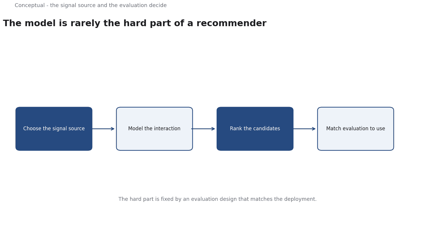
Recommender systems are usually introduced as two approaches — collaborative filtering and content-based filtering — and then a hybrid is mentioned to cover the cases where neither works. That framing is tidy and slightly wrong, because it describes how the features are computed rather than what the system is trying to learn, and it hides the fact that the hard part is rarely the model.
Direct answer: Recommenders learn a relationship between a user and an item, and they differ in where that relationship comes from. Collaborative methods learn it from what users did with each other; content-based methods learn it from the attributes of the items; hybrid methods combine both. The published work on modern recommenders is largely about encoding the interaction structure explicitly and about feature interactions in ranking models. The hard part in practice is not the architecture — it is that offline metrics and online outcomes disagree, and that most of the apparent accuracy comes from the split you chose.
Where the signal comes from
Collaborative filtering learns from behaviour alone. Users who consumed the same items are treated as similar, and an item is recommended because similar users consumed it. Its strength is that it requires no product metadata at all, which is why it still dominates in domains with rich interaction logs and sparse product descriptions. Its weakness is that it cannot recommend anything to a user with no history — the cold-start problem.
Content-based filtering learns from the item itself. A product's attributes, a document's text, a video's metadata are turned into a representation, and the recommendation is for items similar to what the user liked. Its strength is that it works on the first session, when collaborative filtering has nothing to say. Its weakness is that it recommends more of the same, and it can only recommend from the catalogue it knows how to describe.
Hybrid systems use both, usually by combining scores or by feeding both feature families into one model. Guo et al. describe the rationale in terms of feature interactions: "Learning sophisticated feature interactions behind user behaviors is critical in maximizing CTR", and their model is built so that "it is possible to derive an end-to-end learning model that emphasizes both low- and high-order feature interactions". Their evaluation covers "both benchmark data and commercial data", which is the right instinct and rarely done.
The problem the deep models were solving
Matrix factorisation was the dominant approach for years: represent users and items as vectors in a shared space, and predict the missing entries. It works well, and it fails in a specific, identifiable way.
Wang et al. state the failure precisely. The existing approach, "ranging from early matrix factorization to recently emerged deep learning based methods", obtains a user's or item's embedding "by mapping from pre-existing features that describe the user (or the item), such as ID and attributes". The drawback they identify is that "the collaborative signal, which is latent in user-item interactions, is not encoded in the embedding process" — so "the resultant embeddings may not be sufficient to capture the collaborative filtering effect".
That is a precise statement of what was missing. A matrix factorisation model does use interactions, but only as the reconstruction target; the embedding function itself is blind to the graph. NGCF's proposal is to change that: "integrate the user-item interactions -- more specifically the bipartite graph structure -- into the embedding process", so that the representation itself is shaped by the interaction structure rather than only by the fit.
The practical significance is that it moves collaborative signal from the loss into the representation, and it is the step that made graph-based recommenders competitive with well-tuned matrix factorisation rather than a curiosity.
Ranking is a different problem from recommendation
The two problems get conflated, and they have different failure modes.
Recommendation asks: which items should this user see? The candidate set may be the whole catalogue, and the answer is a set.
Ranking asks: given a candidate set, in what order? The candidate set has already been narrowed — usually by a retrieval stage — and the answer is an ordering.
The second is where modern models operate, and it is where the business metric lives. Click-through rate is the objective, and the modelling problem in CTR prediction is the interaction between features: a user's history, the item's attributes, the context, and the combinations of all three.
The two-level architecture has a consequence worth stating plainly. Retrieval and ranking optimise different objectives, and the properties of the final list are decided by both. A system with excellent ranking and mediocre retrieval shows excellent numbers in an offline CTR test and disappointing results in production, because the ranked items are the wrong items.
Where the evaluation breaks
Offline evaluation for recommenders is notoriously fragile, and the reason is worth being precise about: the metrics are computed over a split you chose, and the metrics are not the business objective.
If your data has a time dimension — and it does, because users accumulate interactions — a random split lets the model learn from the future. scikit-learn's TimeSeriesSplit exists for exactly this reason, and its documented behaviour shows why the ordering matters: the default folds are expanding, with fold 0 training on index [0 1 2 3 4 5] and testing on [6 7], fold 1 training on [0 1 2 3 4 5 6 7] and testing on [8 9]. Every training fold is strictly in the past relative to its test fold.
The gap parameter is the detail most teams skip. It inserts a period between the end of the training window and the start of the test window, and the documented example "add[s] a 2 period gap". Without a gap, you are evaluating on a test period that starts immediately after training, which flatters any model that benefits from recency in a way that will not survive deployment.
Beyond the split, three habits produce misleading evaluations. Splitting by user rather than by time measures generalisation to new users while your production system mostly serves existing ones — a mismatch in the wrong direction. Reporting a single aggregate metric hides the segment where the model is actually failing. And evaluating on the items the production retrieval stage already selected measures the ranker, not the system.
None of this is fixable by a better model.
It is fixed by an evaluation design that matches the deployment, which is why the evaluation step usually deserves more attention than the architecture step.
Cold start is a standing constraint
New users and new items break collaborative methods by construction, and the problem never fully disappears because a catalogue is a stream rather than a set. The strategies, their costs, and a worked onboarding example are covered in Cold Start in Recommender Systems, which treats that question in depth. For the present purpose, the point is that a recommender evaluated on a static snapshot is being evaluated on a condition that will not hold in production — so the time-ordered split below is not optional.
A decision sequence that works
- Pick the metric you will be judged on, and find an offline proxy for it. If the business metric is revenue or retention, say so; if you use CTR as a proxy, write down the proxy's limits rather than pretending it is the metric.
- Build the time-ordered split before the model. Expanding or rolling windows, with a gap for the delay between an interaction and its label. If you cannot write the split code today, your offline numbers will be wrong in a way you will not detect.
- Start with the simplest strong baseline — matrix factorisation or a well-tuned collaborative model — and only move to a graph or deep architecture when it beats that baseline on a split you trust.
- Separate retrieval from ranking, and measure each. If the retrieval stage is dropping the answer, no ranker will fix it.
- For content-based components, check the metadata is actually descriptive. The most common failure is a genre string that says nothing, which produces confident, useless recommendations.
- Instrument the segments — new users, new items, and the tail of long-tail items — before you trust the aggregate.
- Plan for the catalogue to move. New-item latency, index freshness, and how quickly a new item can accumulate enough signal to be recommended fairly.
For the ranking objective in a search or ads context, see Search Recommender Engines; for the graph machinery behind interaction-aware embeddings, see Graph Neural Networks.
A worked example
The following is hypothetical and illustrative. Consider a hypothetical catalogue with six months of interaction logs and a ranker to be shipped. Three checks follow from the evaluation advice. First, build a time-ordered split before the model: using the scikit-learn TimeSeriesSplit pattern, assume expanding folds train on the first eight weeks and test on the next week, with the documented gap inserted to stand in for the delay between an interaction and its label; a random split would let the model learn from the future. Second, separate retrieval from ranking and measure each; suppose the retrieval stage keeps only a top-50 candidate set, so a ranker tested on those same 50 items can look strong offline while the right item never reaches it in production. Third, instrument segments - new users, new items, and the long tail - because a single aggregate CTR hides the failing group. The bounded outcome: the offline number drops once the split is honest and the gap included, and the team ships the simpler baseline until the gain survives the time-ordered test. No real catalogue or product is implied.
A counterargument
A reasonable critic would note that the article blames offline evaluation for the gap to online outcomes, while its cited scikit-learn source describes only cross-validation mechanics, not evidence that a correct split predicts production behaviour. A time-ordered split with a gap can be executed flawlessly and still miss the feedback loop the article itself implies: recommendations change the interactions that train the next model, and neither the feature-interaction nor the graph-embedding sources address that. By saying most apparent accuracy comes from the split chosen, the article risks implying that a clean split closes the disagreement, when its own framing treats offline and online as different problems.
The evaluation advice is sound; its status as the usual bottleneck is asserted rather than shown.
References & Further Reading
- Steffen Rendle et al., 2012. Neural Graph Collaborative Filtering — Graph collaborative filtering that propagates over the user-item graph.
- Ruibin Gai et al., 2017. DeepFM: A Factorization-Machine based Neural Network for CTR Prediction — Feature interactions in click-through-rate models, the shared core of search and recommendation ranking.
- scikit-learn developers, 2026. Cross-validation: evaluating estimator performance (scikit-learn) — Time-series splits and the validation design that keeps a backtest honest.