Test-Time Compute: Why Reasoning Models Spend More at Inference
More thinking at answer time can beat a bigger model. Read the research, a worked budget, and when the trade-off pays.
For years, better performance meant a bigger model. A recent line of work shows that spending more compute at inference — searching, sampling, or refining before answering — can be more effective than adding parameters, at least on some tasks. That shifts part of the cost from training to every request.
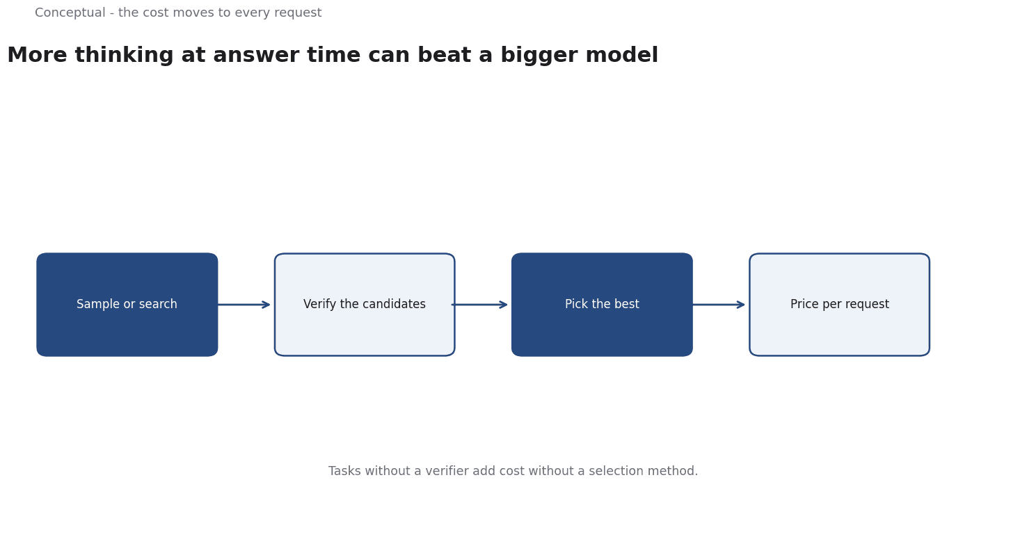
Direct answer: Test-time compute uses additional inference-time work — longer chains of thought, parallel samples, or search over candidate answers — to improve a response. The paper Scaling LLM Test-Time Compute Optimally reports that on certain tasks this outperforms parameter scaling. The boundary: the gain is task-dependent and the cost is per request, so a method that is economical for a rare hard question may be wasteful for high-volume simple ones.
What counts as test-time compute
Three forms are common:
Longer reasoning traces. The model generates more intermediate steps before answering, which the reasoning-model article covers.
Parallel sampling. Generate several candidate answers and select the best, using a verifier or a vote. This trades tokens for a better chance of a correct answer.
Search. Explore a tree of possible reasoning paths, scoring and backtracking. This is the most expensive and most structured form.
They share a principle: use computation at answer time to compensate for a model that is not certain.
A worked budget comparison
The following uses published list prices with hypothetical volumes.
OpenAI lists GPT-6 Astra at $10 input and $50 output per million tokens. A hard question averages 2,000 input tokens.
- Single answer: 500 output tokens → 0.5 × $50/M = $0.025 output; total about $0.045.
- Four parallel samples with verification: 4 × 500 = 2,000 output tokens → $0.10 output, plus a verifier call. Total roughly $0.13 — about three times the cost.
- A larger model with one answer: suppose it costs $20/$80 per million. Input $0.04 + output $0.04 = $0.08, with no extra inference work.
Three lessons follow:
- The comparison depends on the task. If four samples raise accuracy from 70% to 90%, the tripled cost may be worth it. If the gain is two points, it is not.
- Cost moves from training to usage. A smaller model with heavy test-time compute has a low fixed cost and a high marginal cost, which favours low-volume, high-value work.
- There is a crossover point. At very high volume, a larger model with one pass may be cheaper than a smaller model with four, as the routing and cost-estimator articles explain.
Where it pays
Hard, infrequent questions — complex analysis, mathematics, or multi-step planning where a wrong answer is expensive.
Tasks with a verifiable answer. If you can check correctness — a unit test, a calculated result, a schema — parallel sampling and selection work well.
Applications with low latency requirements where extra seconds are acceptable.
Where it does not
High-volume, simple requests. Classification and extraction do not benefit from more thinking, as the task taxonomy explains.
Latency-critical interfaces. A user waiting for a chat reply experiences the extra work as a slower product.
The method is available now, and the choice is whether it fits this workload and budget.
The counterargument — that models will get better and make test-time compute unnecessary — is plausible and misses the current decision.
Measuring whether it works
The only reliable evidence is a comparison on your own workload. Three measurements matter:
Accuracy per unit of compute. Compare accuracy at a fixed budget — say, the cost of one answer — across strategies. A method that raises accuracy but costs five times as much may lose on this measure, as the cost-estimator article explains.
Cost per correct answer. Divide the total spend by the number of correct answers, not the number of requests. This metric makes the trade-off visible when error rates differ.
Latency distribution. Report the tail, not the average. A method that makes 95% of requests fast and 5% very slow may still break a user interface that waits for the slow ones, which the observability article covers.
Run each comparison on a labelled held-out set so the result cannot be an artefact of tuning, as the evaluation article recommends.
What the research does not promise
Not universal superiority. The paper reports gains on specific tasks. A rank on those tasks is not a guarantee for yours, as the benchmarks article argues.
Not free accuracy. More compute raises cost and latency on every request, which changes the unit economics.
Not a replacement for evaluation. Whether the extra compute helps your system is an empirical question, answered by the harness described in the evaluation article.
A decision test
- Classify the task — hard and infrequent, or simple and high-volume?
- Check for a verifier that can select among candidate answers.
- Price the single-answer baseline at your real volume.
- Measure accuracy gain from sampling or longer traces on a labelled set.
- Compute cost per correct answer, not per request.
- Check latency against product expectations.
- Route selectively — extra compute only where it pays.
For the mechanism, see Reasoning Models; for the routing decision, see Routing Between LLMs.
References & Further Reading
- Charlie Snell et al., 2024. Scaling LLM Test-Time Compute Optimally can be More Effective than Scaling Model Parameters — Test-time compute can outperform parameter scaling on some tasks by searching or refining at inference.
- Jason Wei et al., 2022. Chain-of-Thought Prompting Elicits Reasoning in Large Language Models — The paper showing that generating intermediate reasoning steps improves performance on reasoning tasks.