Time Series Forecasting: ARIMA, Prophet, and Deep Learning Models
Forecasting methods make different assumptions about what drives the future. Read the mechanism behind ARIMA, modern hurtles, and neural forecasters — and how to choose.
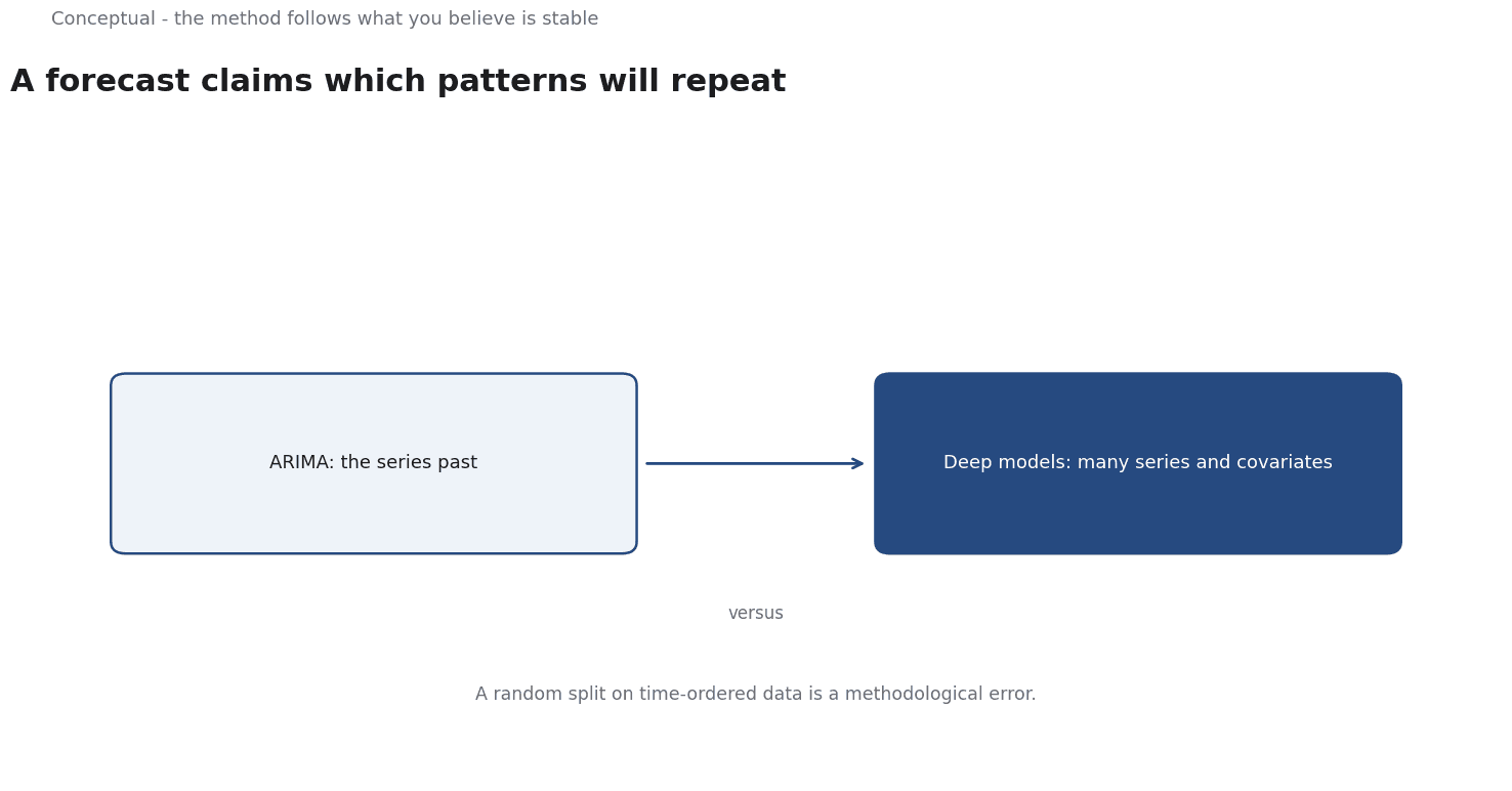
A time series forecast is a claim about which patterns will repeat. ARIMA assumes structure in the series itself; models with regressors assume external variables help; neural forecasters assume there is a learnable mapping from history and covariates to the future. None of these is universally right, and the choice is mostly a question of what you believe is stable.
Direct answer: Classical methods such as exponential smoothing and ARIMA model the series from its own past and work well on short, relatively clean series with clear patterns. Deep models such as N-BEATS and the Temporal Fusion Transformer learn from large collections of series and can incorporate covariates, at the cost of data and complexity. Oreshkin et al. report that N-BEATS improved forecast accuracy by 11% over a statistical benchmark and 3% over the previous M4 competition winner, so the neural approach is genuinely competitive — but that result is on competition datasets, not a guarantee for a single business series.
What makes time series different
A row in a time series is not independent of the row before it. This breaks the usual cross-validation assumption and introduces three issues that must be handled explicitly.
Trend and seasonality. A series can drift upward and repeat a daily or yearly cycle. A model that treats these as noise will waste capacity relearning them.
Non-stationarity. The statistical properties of the series can change. A model fitted on last year's data may describe a process that no longer exists — the reason a forecast can fail without any bug in the code.
Leakage from the future. Randomly splitting a time series lets the model see observations that occur after the ones it is predicting. scikit-learn's TimeSeriesSplit exists for this reason: it builds expanding folds that respect chronology, and its gap parameter handles cases where labels arrive late.
The forecasting textbook Forecasting: Principles and Practice by Hyndman and Athanasopoulos is the clearest reference for the classical toolkit — exponential smoothing, ARIMA, and the discipline of evaluating on a holdout that mimics the deployment horizon.
The classical approach
ARIMA models a series as a function of its own past values and past errors. The "AR" term captures dependence on previous observations; the "MA" term captures dependence on previous forecast errors; "I" denotes differencing, which removes trend to make the series stationary.
The appeal is transparency and low data requirements. On a single series with a few hundred observations and a stable pattern, an ARIMA or exponential-smoothing model is often hard to beat, and its assumptions can be checked.
The limitation is that a univariate model ignores everything else. If promotions, holidays, or price changes drive demand, the series alone is an incomplete description, and no amount of tuning recovers information that was never in the inputs.
The deep learning approach
Deep forecasters address two weaknesses at once: they can share information across many related series, and they can incorporate covariates.
N-BEATS, from Oreshkin et al., is built from "backward and forward residual links and a very deep stack of fully-connected layers". Its basis-expansion design makes the output decomposable — the forecast can be expressed as trend and seasonality components — which is what the authors mean by interpretable. The paper tested it on M3, M4, and TOURISM datasets and reported state-of-the-art results, with an 11% improvement over a statistical benchmark and 3% over the previous M4 winner, a hand-crafted hybrid model.
The Temporal Fusion Transformer, from Lim et al., targets multi-horizon forecasting with a "complex mix of inputs — including static covariates, known future inputs, and other exogenous time series that are only observed historically". It combines "recurrent layers for local processing and interpretable self-attention layers for learning long-term dependencies" and produces variable-importance measures, which matter when a human needs to trust a forecast.
The distinction between covariate types is practically important. A known future input — a planned promotion, a holiday calendar — can be used directly. A covariate observed only historically — yesterday's actual traffic — must be forecast or lagged, and treating it as known is a subtle form of leakage.
A worked example of horizon and validation
Suppose you need a daily demand forecast for the next 14 days, using two years of history.
A correct validation design uses a rolling origin: train on the first 700 days, forecast days 701–714, measure error; then train on 714 days, forecast days 715–728; repeat. Each fold mirrors the real task — predicting 14 days ahead with only past data available.
Now add a planned promotion in week 3 of the forecast. This is a known future covariate, so a model that accepts calendar features can use it. A univariate ARIMA cannot; it will treat the promotion's effect as unexplained error and, if the promotion recurs, may eventually learn a seasonal pattern that only coincidentally aligns.
The choice between a "simple" and a "powerful" model depends on this detail. With 20 related product series and a promotion calendar, a shared deep model with covariates can exploit information a set of independent ARIMA fits cannot. With one series, no covariates, and 400 observations, the deep model has nothing to learn from that the classical model does not already see.
The arithmetic of error also matters. A 5% mean absolute percentage error is meaningless if the series contains zeros or near-zeros; use a scale-dependent measure with a stated denominator, and report error by segment, since aggregate accuracy can hide systematic failure on the products that matter most.
What the competition results do not tell you
Three caveats change the practical conclusion.
Competition datasets are not your data. M4 and TOURISM contain thousands of diverse series. A method that wins there benefits from cross-series learning; if you have one series, that advantage disappears.
Accuracy is not the only criterion. N-BEATS and TFT are described as interpretable relative to earlier neural models, but an ARIMA coefficient or an exponential-smoothing component is still easier to explain to a stakeholder. In a setting where a human must act on the forecast, a small accuracy gain may not justify the loss of transparency.
Any model assumes the future resembles the past in relevant ways.
The world moves. A structural break — a new competitor, a policy change — invalidates the historical relationship regardless of architecture. Monitoring forecast error and retraining on a schedule is part of the method, not an afterthought.
A decision test
- State the horizon and the covariate availability before choosing a model.
- Build a naive or seasonal-naive baseline and a simple exponential-smoothing or ARIMA model.
- Validate with a rolling origin that mirrors the deployment horizon, never a random split.
- Add covariates only if they are genuinely available at prediction time.
- Move to a deep model when you have many related series, rich covariates, or clear evidence that the baselines leave structured error on the table.
- Report error by segment with explicit denominators, and monitor it after deployment.
For the validation and monitoring discipline that makes any of this trustworthy, see Model Monitoring; for the operational side, see MLOps.
For a worked example that treats the prediction moment as a variable and compares seven models over 133 out-of-sample months, see the BTC Monthly ML case study; it shows why late-month accuracy is descriptive rather than tradable.
A counterargument
A reasonable critic would say the article's balanced framing still flatters the deep models. It cites N-BEATS's 11% and 3% gains as evidence the neural approach is "genuinely competitive," then notes these come from competition datasets with thousands of series - which is the article's own explanation for why the advantage disappears on a single series. The classical toolkit is defended with Hyndman's text, while the deep models are defended with competition win rates, and those are different kinds of evidence. scikit-learn's TimeSeriesSplit validates a backtest design, not a choice of model. The decision test is sensible, but the framing invites an inference - that deep models win on benchmarks - that the article's own caveats are meant to retract.
The headline number is the one readers remember; the caveat is the one they skip.
References & Further Reading
- Rob J. Hyndman and George Athanasopoulos, 2013. Forecasting: Principles and Practice (2nd edition) — The free standard text on forecasting practice, evaluation, and error measures.
- Boris Oreshkin et al., 2020. N-BEATS: Neural Basis Expansion Analysis for Interpretable Time Series Forecasting — A deep forecasting architecture with interpretable basis functions.
- Bryan Lim et al., 2021. Temporal Fusion Transformers for Interpretable Multi-horizon Time Series Forecasting — Static covariates, known future inputs, and variable selection in one architecture.
- scikit-learn developers, 2026. Cross-validation: evaluating estimator performance (scikit-learn) — Time-series splits and the validation design that keeps a backtest honest.